R Graphical Manual

Browse All

Last data update: 2014.03.03

R: scatterplot matrix with potentially different sets of...

xysplom

R Documentation

scatterplot matrix with potentially different sets of variables on the rows and columns.

Description

scatterplot matrix with potentially different sets of variables on the rows and columns. The slope or regression coefficient for simple least squares regression can be displayed in the strip label for each panel.

Usage

xysplom(x, ...)

## S3 method for class 'formula'
xysplom(x, data = sys.parent(), na.action = na.pass, ...)

## Default S3 method:
xysplom(x, y=x, group, relation="free",
        x.relation=relation, y.relation=relation,
        xlim.in=NULL, ylim.in=NULL,
        corr=FALSE, beta=FALSE, abline=corr||beta, digits=3,
        x.between=NULL, y.between=NULL,
        between.in=list(x=x.between, y=y.between),
        scales.in=list(
          x=list(relation=x.relation, alternating=FALSE),
          y=list(relation=y.relation, alternating=FALSE)),
        strip.in=strip.xysplom,
        pch=16, cex=.75,
        panel.input=panel.xysplom, ...,
        cartesian=TRUE,
        plot=TRUE)

Arguments

`x`	In the `"formula"` method, a formula. In the `"default"` method, a data.frame. Any variables that are used in a formula with `+` should be numeric. Factors are not rejected, but their levels will be combined strangely.
`...`	other arguments to `xyplot`.

`data`	data.frame
`na.action`	See `na.action`. Defaults to `na.pass` because `xyplot` does sensible things with missing data.

`y`	In the `"default"` method, a data.frame with the same number of rows as the data.frame in `x`.
`group`	In the `"default"` method, a data.frame with the same number of rows as the data.frame in `x`.
`relation, x.relation, y.relation,scales.in`	Alternate ways to get to the `scales(relation=)` arguments to `xyplot`.
`xlim.in, ylim.in`	Alternate ways to get to the `scales(limits=)` arguments to `xyplot`.
`corr, beta`	Display the correlation and/or the regression coefficient for `lm(y ~ x)` for each panel in an additional strip label.
`abline`	logical. If `TRUE`, draw the least squares regression line within each panel. By default the abline is `FALSE` unless at least one of `corr` or `beta` is `TRUE`.
`digits`	number of significant digits for the correlation coefficient.
`x.between, y.between, between.in`	Alternate ways to get to the `between=` argument to `xyplot`.
`strip.in`	strip function that knows how to handle the `corr` and `beta` displays.
`pch, cex`	arguments to `xyplot`
`panel.input`	panel function used by `xyplot` within each panel. When `abline==FALSE`, the default panel function calls `panel.xyplot`. When `abline==TRUE`, the default panel function calls `panel.xyplot` and `panel.abline(lm(y~x, na.action=na.exclude))`. Note that we use `na.action=na.exclude` inside `lm`.
`cartesian`	When `cartesian==TRUE`, the cartesian product of the left-hand side number of variables and the right-hand side number of variables defines the number of panels in the display. When `cartesian==FALSE`, each variable in the left-hand side is paired with the variable in the corresponding position in the right-hand side and only those pairs are plotted. Both sides must have the same number of variables.
`plot`	Defaults to `TRUE`. See details.

Details

The argument plot=TRUE is the normal setting and then the function returns a "trellis" object. When the argument plot=FALSE, the function returns the argument list that would otherwise be sent to xyplot. This list is interesting when the function xysplom was designed because the function works by restructuring the input data and running xyplot on the restructured data.

Value

When plot=TRUE (the normal setting), the "trellis" object containing the graph.
When plot=FALSE, the restructured data that must be sent to the xyplot function.

Author(s)

Richard M. Heiberger <rmh@temple.edu>

References

Heiberger, Richard M. and Holland, Burt (2004b). Statistical Analysis and Data Display: An Intermediate Course with Examples in S-Plus, R, and SAS. Springer Texts in Statistics. Springer. ISBN 0-387-40270-5.

Examples


## xysplom syntax options

tmp <- data.frame(y=rnorm(12), x=rnorm(12), z=rnorm(12), w=rnorm(12),
                  g=factor(rep(1:2,c(6,6))))
tmp2 <- tmp[,1:4]

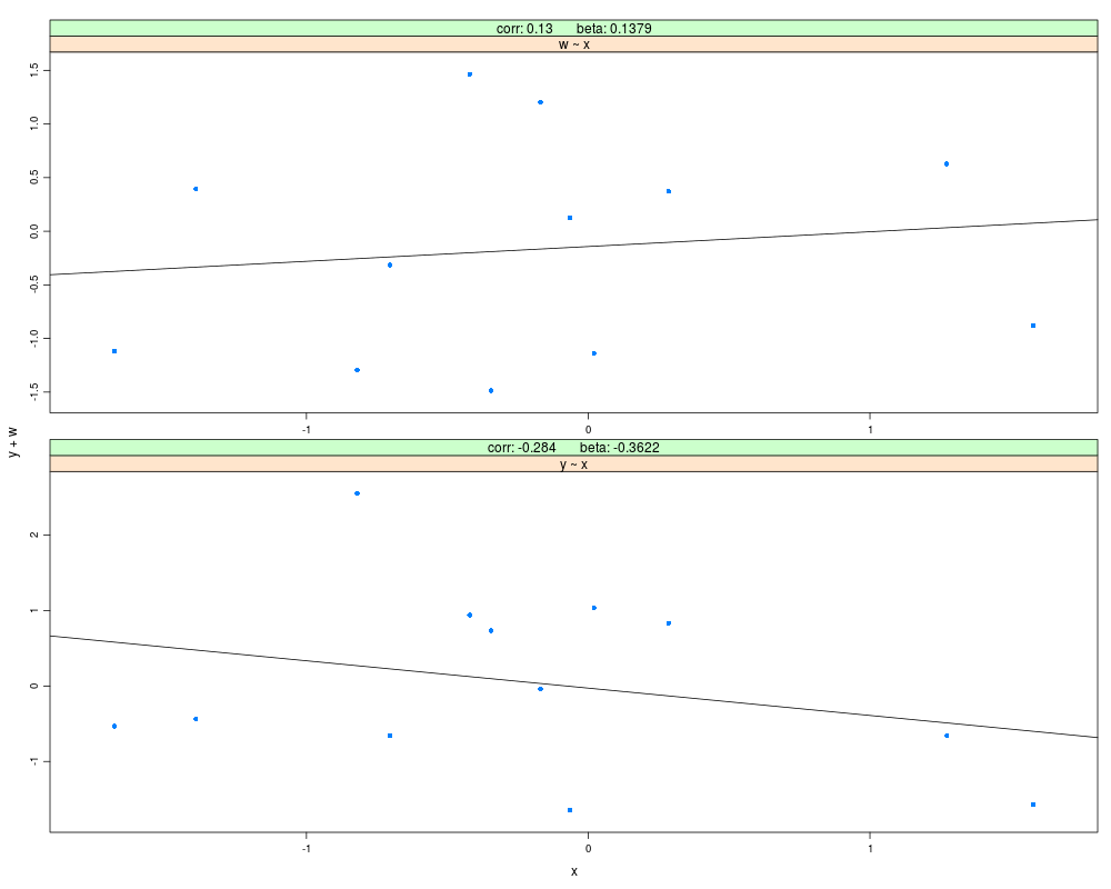
xysplom(y + w ~ x , data=tmp, corr=TRUE, beta=TRUE, cartesian=FALSE, layout=c(1,2))

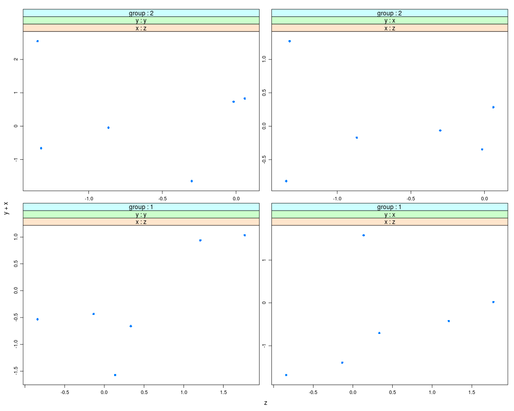
xysplom(y + x ~ z | g, data=tmp, layout=c(2,2))
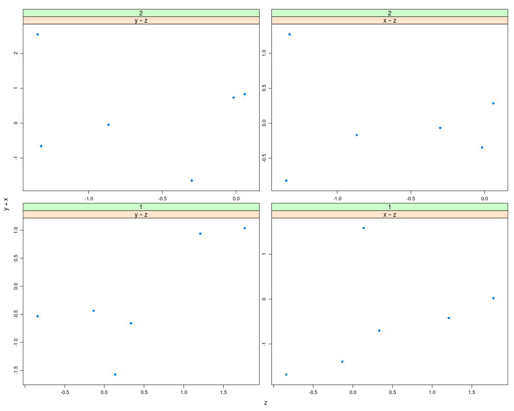
xysplom(y + x ~ z | g, data=tmp, cartesian=FALSE)

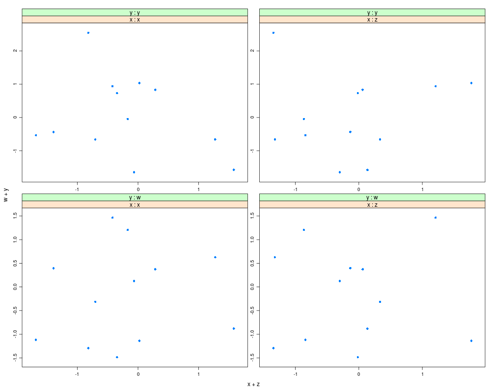
xysplom(w + y ~ x + z, data=tmp)
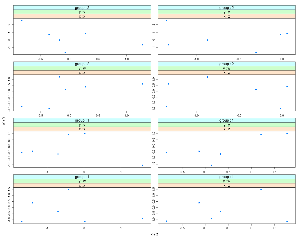
xysplom(w + y ~ x + z | g, data=tmp, layout=c(2,4))
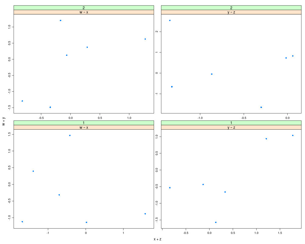
xysplom(w + y ~ x + z | g, data=tmp, cartesian=FALSE)

## Not run: 
## xyplot in R has many similar capabilities with xysplom
if.R(r=
       xyplot(w + z ~ x + y, data=tmp, outer=TRUE)
     ,s=
       {}
    )

## End(Not run)

Results


R version 3.3.1 (2016-06-21) -- "Bug in Your Hair"
Copyright (C) 2016 The R Foundation for Statistical Computing
Platform: x86_64-pc-linux-gnu (64-bit)

R is free software and comes with ABSOLUTELY NO WARRANTY.
You are welcome to redistribute it under certain conditions.
Type 'license()' or 'licence()' for distribution details.

R is a collaborative project with many contributors.
Type 'contributors()' for more information and
'citation()' on how to cite R or R packages in publications.

Type 'demo()' for some demos, 'help()' for on-line help, or
'help.start()' for an HTML browser interface to help.
Type 'q()' to quit R.

> library(HH)
Loading required package: lattice
Loading required package: grid
Loading required package: latticeExtra
Loading required package: RColorBrewer
Loading required package: multcomp
Loading required package: mvtnorm
Loading required package: survival
Loading required package: TH.data
Loading required package: MASS

Attaching package: 'TH.data'

The following object is masked from 'package:MASS':

    geyser

Loading required package: gridExtra
> png(filename="/home/ddbj/snapshot/RGM3/R_CC/result/HH/xysplom.Rd_%03d_medium.png", width=480, height=480)
> ### Name: xysplom
> ### Title: scatterplot matrix with potentially different sets of variables
> ###   on the rows and columns.
> ### Aliases: xysplom xysplom.formula xysplom.default
> ### Keywords: hplot
> 
> ### ** Examples
> 
> 
> ## xysplom syntax options
> 
> tmp <- data.frame(y=rnorm(12), x=rnorm(12), z=rnorm(12), w=rnorm(12),
+                   g=factor(rep(1:2,c(6,6))))
> tmp2 <- tmp[,1:4]
> 
> xysplom(y + w ~ x , data=tmp, corr=TRUE, beta=TRUE, cartesian=FALSE, layout=c(1,2))
> 
> xysplom(y + x ~ z | g, data=tmp, layout=c(2,2))
> xysplom(y + x ~ z | g, data=tmp, cartesian=FALSE)
> 
> xysplom(w + y ~ x + z, data=tmp)
> xysplom(w + y ~ x + z | g, data=tmp, layout=c(2,4))
> xysplom(w + y ~ x + z | g, data=tmp, cartesian=FALSE)
> 
> ## Not run: 
> ##D ## xyplot in R has many similar capabilities with xysplom
> ##D if.R(r=
> ##D        xyplot(w + z ~ x + y, data=tmp, outer=TRUE)
> ##D      ,s=
> ##D        {}
> ##D     )
> ## End(Not run)
> 
> 
> 
> 
> 
> 
> dev.off()
null device 
          1 
>