Function to perform Adaptive Rejection Metropolis Sampling

Description

Generates a sequence of random variables using ARMS. For multivariate densities, ARMS is used along randomly selected straight lines through the current point.

Usage

arms(y.start, myldens, indFunc, n.sample, ...)

Arguments

Details

Strictly speaking, the support of the target density must be a bounded convex set. When this is not the case, the following tricks usually work. If the support is not bounded, restrict it to a bounded set having probability practically one. A workaround, if the support is not convex, is to consider the convex set generated by the support and define myldens to return log(.Machine$double.xmin) outside the true support (see the last example.)

The next point is generated along a randomly selected line through the current point using arms.

Make sure the value returned by myldens is never smaller than log(.Machine$double.xmin), to avoid divisions by zero.

Value

An n.sample by length(y.start) matrix, whose rows are the sampled points.

Note

The function is based on original C code by Wally Gilks for the univariate case, http://www.mrc-bsu.cam.ac.uk/pub/methodology/adaptive_rejection/.

Author(s)

Giovanni Petris GPetris@uark.edu

References

Gilks, W.R., Best, N.G. and Tan, K.K.C. (1995) Adaptive rejection Metropolis sampling within Gibbs sampling (Corr: 97V46 p541-542 with Neal, R.M.), Applied Statistics 44:455–472.

Examples

#### ==> Warning: running the examples may take a few minutes! <== ####    
### Univariate densities
## Unif(-r,r) 
y <- arms(runif(1,-1,1), function(x,r) 1, function(x,r) (x>-r)*(x<r), 5000, r=2)
summary(y); hist(y,prob=TRUE,main="Unif(-r,r); r=2")
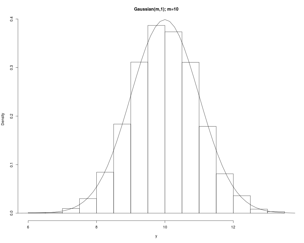
## Normal(mean,1)
norldens <- function(x,mean) -(x-mean)^2/2 
y <- arms(runif(1,3,17), norldens, function(x,mean) ((x-mean)>-7)*((x-mean)<7),
          5000, mean=10)
summary(y); hist(y,prob=TRUE,main="Gaussian(m,1); m=10")
curve(dnorm(x,mean=10),3,17,add=TRUE)
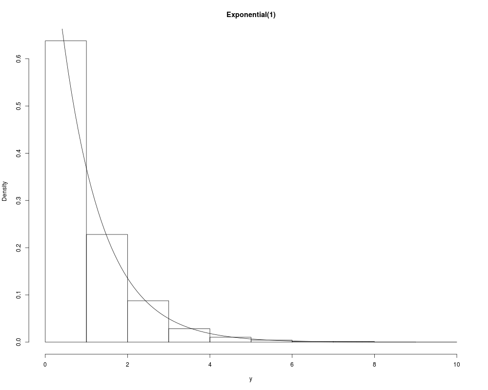
## Exponential(1)
y <- arms(5, function(x) -x, function(x) (x>0)*(x<70), 5000)
summary(y); hist(y,prob=TRUE,main="Exponential(1)")
curve(exp(-x),0,8,add=TRUE)
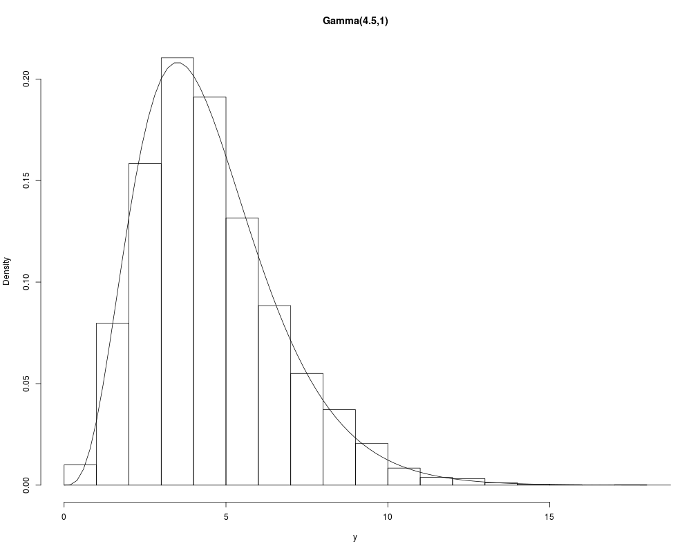
## Gamma(4.5,1) 
y <- arms(runif(1,1e-4,20), function(x) 3.5*log(x)-x,
          function(x) (x>1e-4)*(x<20), 5000)
summary(y); hist(y,prob=TRUE,main="Gamma(4.5,1)")
curve(dgamma(x,shape=4.5,scale=1),1e-4,20,add=TRUE)
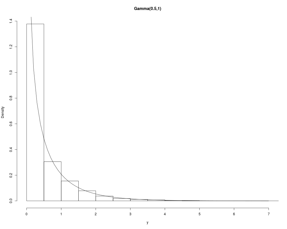
## Gamma(0.5,1) (this one is not log-concave)
y <- arms(runif(1,1e-8,10), function(x) -0.5*log(x)-x,
          function(x) (x>1e-8)*(x<10), 5000)
summary(y); hist(y,prob=TRUE,main="Gamma(0.5,1)")
curve(dgamma(x,shape=0.5,scale=1),1e-8,10,add=TRUE)
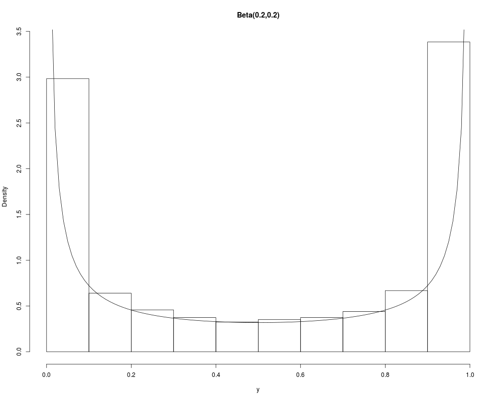
## Beta(.2,.2) (this one neither)
y <- arms(runif(1), function(x) (0.2-1)*log(x)+(0.2-1)*log(1-x),
          function(x) (x>1e-5)*(x<1-1e-5), 5000)
summary(y); hist(y,prob=TRUE,main="Beta(0.2,0.2)")
curve(dbeta(x,0.2,0.2),1e-5,1-1e-5,add=TRUE)
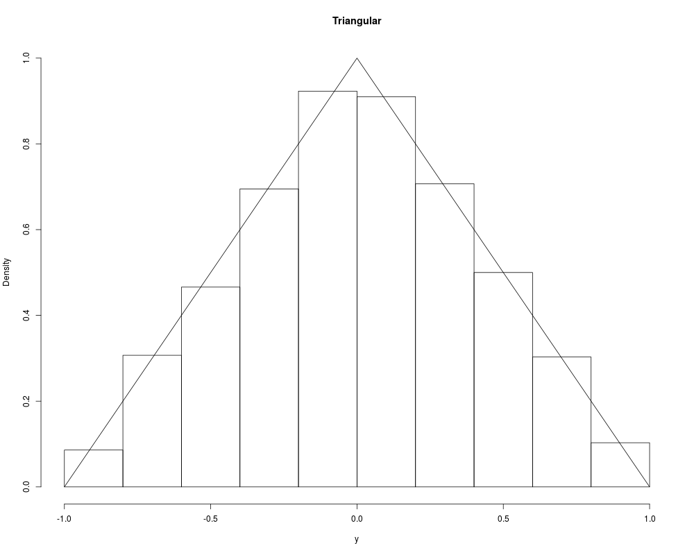
## Triangular
y <- arms(runif(1,-1,1), function(x) log(1-abs(x)), function(x) abs(x)<1, 5000)     
summary(y); hist(y,prob=TRUE,ylim=c(0,1),main="Triangular")
curve(1-abs(x),-1,1,add=TRUE)
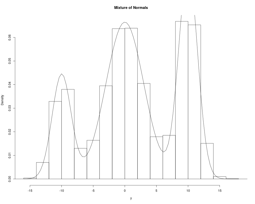
## Multimodal examples (Mixture of normals)
lmixnorm <- function(x,weights,means,sds) {
    log(crossprod(weights, exp(-0.5*((x-means)/sds)^2 - log(sds))))
}
y <- arms(0, lmixnorm, function(x,...) (x>(-100))*(x<100), 5000, weights=c(1,3,2),
          means=c(-10,0,10), sds=c(1.5,3,1.5))
summary(y); hist(y,prob=TRUE,main="Mixture of Normals")
curve(colSums(c(1,3,2)/6*dnorm(matrix(x,3,length(x),byrow=TRUE),c(-10,0,10),c(1.5,3,1.5))),
      par("usr")[1], par("usr")[2], add=TRUE)

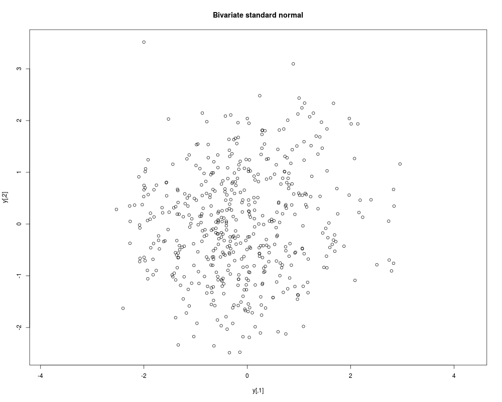
### Bivariate densities 
## Bivariate standard normal
y <- arms(c(0,2), function(x) -crossprod(x)/2,
          function(x) (min(x)>-5)*(max(x)<5), 500)
plot(y, main="Bivariate standard normal", asp=1)
## Uniform in the unit square
y <- arms(c(0.2,.6), function(x) 1,
          function(x) (min(x)>0)*(max(x)<1), 500)
plot(y, main="Uniform in the unit square", asp=1)
polygon(c(0,1,1,0),c(0,0,1,1))
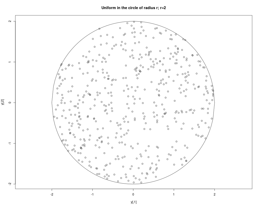
## Uniform in the circle of radius r
y <- arms(c(0.2,0), function(x,...) 1,
          function(x,r2) sum(x^2)<r2, 500, r2=2^2)
plot(y, main="Uniform in the circle of radius r; r=2", asp=1)
curve(-sqrt(4-x^2), -2, 2, add=TRUE)
curve(sqrt(4-x^2), -2, 2, add=TRUE)
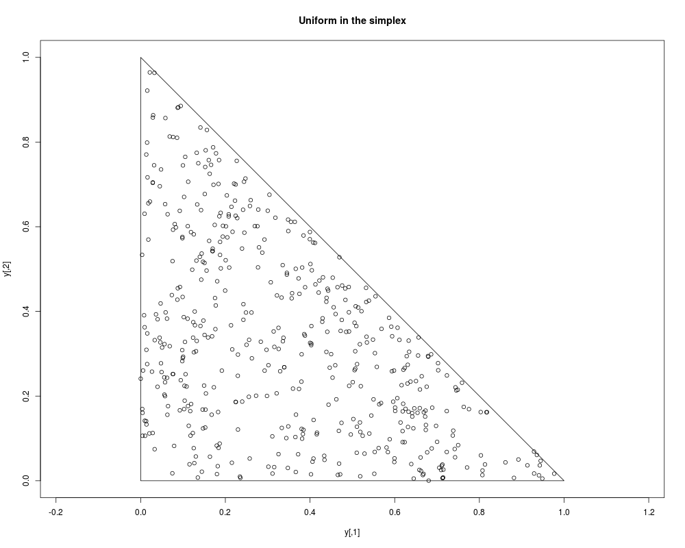
## Uniform on the simplex
simp <- function(x) if ( any(x<0) || (sum(x)>1) ) 0 else 1
y <- arms(c(0.2,0.2), function(x) 1, simp, 500)
plot(y, xlim=c(0,1), ylim=c(0,1), main="Uniform in the simplex", asp=1)
polygon(c(0,1,0), c(0,0,1))
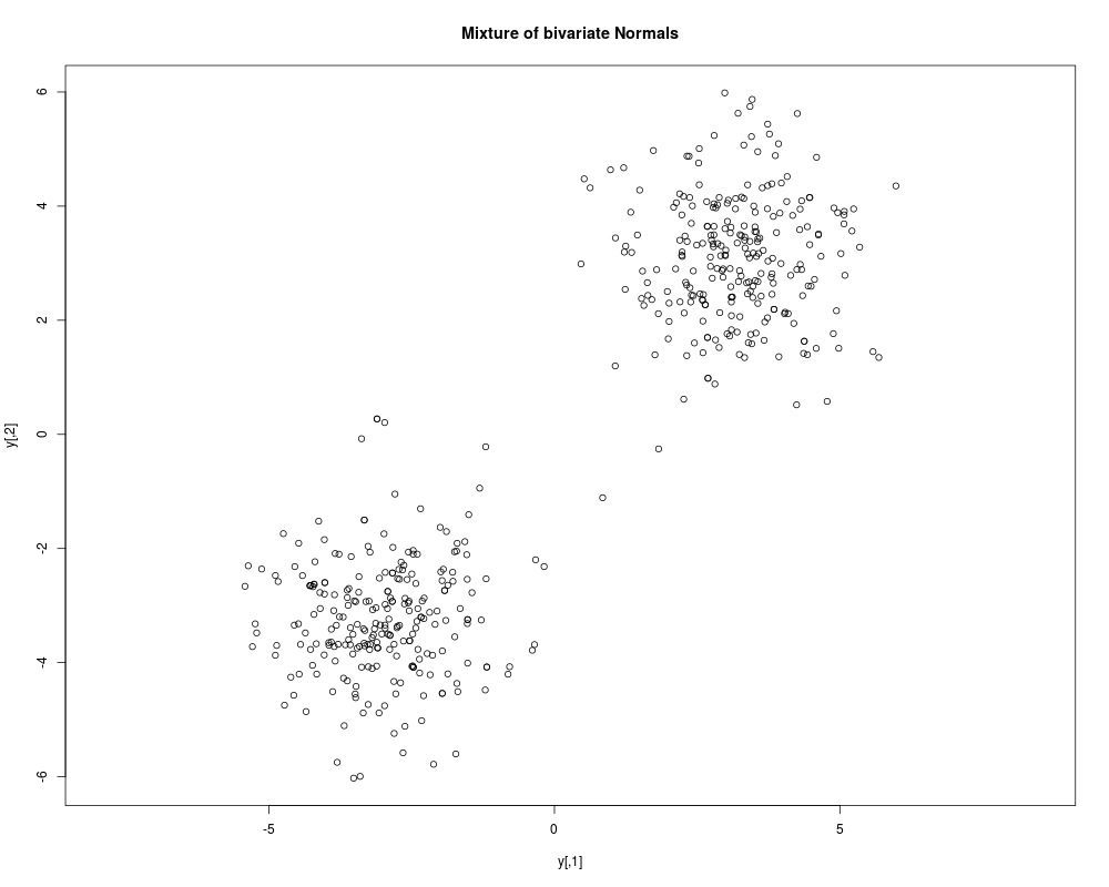
## A bimodal distribution (mixture of normals)
bimodal <- function(x) { log(prod(dnorm(x,mean=3))+prod(dnorm(x,mean=-3))) }
y <- arms(c(-2,2), bimodal, function(x) all(x>(-10))*all(x<(10)), 500)
plot(y, main="Mixture of bivariate Normals", asp=1)

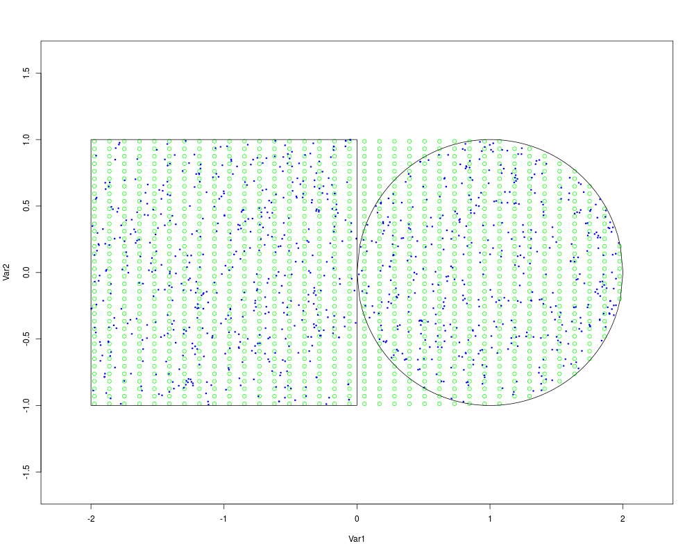
## A bivariate distribution with non-convex support
support <- function(x) {
    return(as.numeric( -1 < x[2] && x[2] < 1 &&
                      -2 < x[1] &&
                      ( x[1] < 1 || crossprod(x-c(1,0)) < 1 ) ) )
}
Min.log <- log(.Machine$double.xmin) + 10
logf <- function(x) {
    if ( x[1] < 0 ) return(log(1/4))
    else
        if (crossprod(x-c(1,0)) < 1 ) return(log(1/pi))
    return(Min.log)
}
x <- as.matrix(expand.grid(seq(-2.2,2.2,length=40),seq(-1.1,1.1,length=40)))
y <- sapply(1:nrow(x), function(i) support(x[i,]))
plot(x,type='n',asp=1)
points(x[y==1,],pch=1,cex=1,col='green')
z <- arms(c(0,0), logf, support, 1000)
points(z,pch=20,cex=0.5,col='blue')
polygon(c(-2,0,0,-2),c(-1,-1,1,1))
curve(-sqrt(1-(x-1)^2),0,2,add=TRUE)
curve(sqrt(1-(x-1)^2),0,2,add=TRUE)
sum( z[,1] < 0 ) # sampled points in the square
sum( apply(t(z)-c(1,0),2,crossprod) < 1 ) # sampled points in the circle

Results

R version 3.3.1 (2016-06-21) -- "Bug in Your Hair"
Copyright (C) 2016 The R Foundation for Statistical Computing
Platform: x86_64-pc-linux-gnu (64-bit)

R is free software and comes with ABSOLUTELY NO WARRANTY.
You are welcome to redistribute it under certain conditions.
Type 'license()' or 'licence()' for distribution details.

R is a collaborative project with many contributors.
Type 'contributors()' for more information and
'citation()' on how to cite R or R packages in publications.

Type 'demo()' for some demos, 'help()' for on-line help, or
'help.start()' for an HTML browser interface to help.
Type 'q()' to quit R.

> library(HI)
> png(filename="/home/ddbj/snapshot/RGM3/R_CC/result/HI/arms.Rd_%03d_medium.png", width=480, height=480)
> ### Name: arms
> ### Title: Function to perform Adaptive Rejection Metropolis Sampling
> ### Aliases: arms
> ### Keywords: distribution multivariate misc
> 
> ### ** Examples
> 
> #### ==> Warning: running the examples may take a few minutes! <== ####    
> ### Univariate densities
> ## Unif(-r,r) 
> y <- arms(runif(1,-1,1), function(x,r) 1, function(x,r) (x>-r)*(x<r), 5000, r=2)
> summary(y); hist(y,prob=TRUE,main="Unif(-r,r); r=2")
    Min.  1st Qu.   Median     Mean  3rd Qu.     Max. 
-2.00000 -0.94740  0.02825  0.00799  0.96660  1.99900 
> ## Normal(mean,1)
> norldens <- function(x,mean) -(x-mean)^2/2 
> y <- arms(runif(1,3,17), norldens, function(x,mean) ((x-mean)>-7)*((x-mean)<7),
+           5000, mean=10)
> summary(y); hist(y,prob=TRUE,main="Gaussian(m,1); m=10")
   Min. 1st Qu.  Median    Mean 3rd Qu.    Max. 
  5.859   9.303   9.996   9.985  10.680  13.450 
> curve(dnorm(x,mean=10),3,17,add=TRUE)
> ## Exponential(1)
> y <- arms(5, function(x) -x, function(x) (x>0)*(x<70), 5000)
> summary(y); hist(y,prob=TRUE,main="Exponential(1)")
    Min.  1st Qu.   Median     Mean  3rd Qu.     Max. 
0.000158 0.285100 0.694900 1.008000 1.418000 8.843000 
> curve(exp(-x),0,8,add=TRUE)
> ## Gamma(4.5,1) 
> y <- arms(runif(1,1e-4,20), function(x) 3.5*log(x)-x,
+           function(x) (x>1e-4)*(x<20), 5000)
> summary(y); hist(y,prob=TRUE,main="Gamma(4.5,1)")
   Min. 1st Qu.  Median    Mean 3rd Qu.    Max. 
 0.4334  2.9570  4.1680  4.4860  5.6890 14.8100 
> curve(dgamma(x,shape=4.5,scale=1),1e-4,20,add=TRUE)
> ## Gamma(0.5,1) (this one is not log-concave)
> y <- arms(runif(1,1e-8,10), function(x) -0.5*log(x)-x,
+           function(x) (x>1e-8)*(x<10), 5000)
> summary(y); hist(y,prob=TRUE,main="Gamma(0.5,1)")
    Min.  1st Qu.   Median     Mean  3rd Qu.     Max. 
0.000035 0.034940 0.209900 0.487300 0.650000 7.101000 
> curve(dgamma(x,shape=0.5,scale=1),1e-8,10,add=TRUE)
> ## Beta(.2,.2) (this one neither)
> y <- arms(runif(1), function(x) (0.2-1)*log(x)+(0.2-1)*log(1-x),
+           function(x) (x>1e-5)*(x<1-1e-5), 5000)
> summary(y); hist(y,prob=TRUE,main="Beta(0.2,0.2)")
     Min.   1st Qu.    Median      Mean   3rd Qu.      Max. 
0.0001326 0.0814000 0.6396000 0.5504000 0.9801000 1.0000000 
> curve(dbeta(x,0.2,0.2),1e-5,1-1e-5,add=TRUE)
> ## Triangular
> y <- arms(runif(1,-1,1), function(x) log(1-abs(x)), function(x) abs(x)<1, 5000)     
> summary(y); hist(y,prob=TRUE,ylim=c(0,1),main="Triangular")
     Min.   1st Qu.    Median      Mean   3rd Qu.      Max. 
-0.981800 -0.284800  0.001771  0.001431  0.298000  0.978700 
> curve(1-abs(x),-1,1,add=TRUE)
> ## Multimodal examples (Mixture of normals)
> lmixnorm <- function(x,weights,means,sds) {
+     log(crossprod(weights, exp(-0.5*((x-means)/sds)^2 - log(sds))))
+ }
> y <- arms(0, lmixnorm, function(x,...) (x>(-100))*(x<100), 5000, weights=c(1,3,2),
+           means=c(-10,0,10), sds=c(1.5,3,1.5))
> summary(y); hist(y,prob=TRUE,main="Mixture of Normals")
   Min. 1st Qu.  Median    Mean 3rd Qu.    Max. 
-14.690  -2.858   1.243   1.580   8.898  15.470 
> curve(colSums(c(1,3,2)/6*dnorm(matrix(x,3,length(x),byrow=TRUE),c(-10,0,10),c(1.5,3,1.5))),
+       par("usr")[1], par("usr")[2], add=TRUE)
> 
> ### Bivariate densities 
> ## Bivariate standard normal
> y <- arms(c(0,2), function(x) -crossprod(x)/2,
+           function(x) (min(x)>-5)*(max(x)<5), 500)
> plot(y, main="Bivariate standard normal", asp=1)
> ## Uniform in the unit square
> y <- arms(c(0.2,.6), function(x) 1,
+           function(x) (min(x)>0)*(max(x)<1), 500)
> plot(y, main="Uniform in the unit square", asp=1)
> polygon(c(0,1,1,0),c(0,0,1,1))
> ## Uniform in the circle of radius r
> y <- arms(c(0.2,0), function(x,...) 1,
+           function(x,r2) sum(x^2)<r2, 500, r2=2^2)
> plot(y, main="Uniform in the circle of radius r; r=2", asp=1)
> curve(-sqrt(4-x^2), -2, 2, add=TRUE)
> curve(sqrt(4-x^2), -2, 2, add=TRUE)
> ## Uniform on the simplex
> simp <- function(x) if ( any(x<0) || (sum(x)>1) ) 0 else 1
> y <- arms(c(0.2,0.2), function(x) 1, simp, 500)
> plot(y, xlim=c(0,1), ylim=c(0,1), main="Uniform in the simplex", asp=1)
> polygon(c(0,1,0), c(0,0,1))
> ## A bimodal distribution (mixture of normals)
> bimodal <- function(x) { log(prod(dnorm(x,mean=3))+prod(dnorm(x,mean=-3))) }
> y <- arms(c(-2,2), bimodal, function(x) all(x>(-10))*all(x<(10)), 500)
> plot(y, main="Mixture of bivariate Normals", asp=1)
> 
> ## A bivariate distribution with non-convex support
> support <- function(x) {
+     return(as.numeric( -1 < x[2] && x[2] < 1 &&
+                       -2 < x[1] &&
+                       ( x[1] < 1 || crossprod(x-c(1,0)) < 1 ) ) )
+ }
> Min.log <- log(.Machine$double.xmin) + 10
> logf <- function(x) {
+     if ( x[1] < 0 ) return(log(1/4))
+     else
+         if (crossprod(x-c(1,0)) < 1 ) return(log(1/pi))
+     return(Min.log)
+ }
> x <- as.matrix(expand.grid(seq(-2.2,2.2,length=40),seq(-1.1,1.1,length=40)))
> y <- sapply(1:nrow(x), function(i) support(x[i,]))
> plot(x,type='n',asp=1)
> points(x[y==1,],pch=1,cex=1,col='green')
> z <- arms(c(0,0), logf, support, 1000)
> points(z,pch=20,cex=0.5,col='blue')
> polygon(c(-2,0,0,-2),c(-1,-1,1,1))
> curve(-sqrt(1-(x-1)^2),0,2,add=TRUE)
> curve(sqrt(1-(x-1)^2),0,2,add=TRUE)
> sum( z[,1] < 0 ) # sampled points in the square
[1] 526
> sum( apply(t(z)-c(1,0),2,crossprod) < 1 ) # sampled points in the circle
[1] 474
> 
> 
> 
> 
> 
> dev.off()
null device 
          1 
>