plotLikelihood( ) plots the likelihood, and plotDiagnostic( ) plots diagnostic-plot of posterior draws of the parameters from MCMC sample. plotHLSM.random.fit( ) and plotHLSM.fixed.fit( ) are functions to plot mean-results from fitted models, and plotHLSM.LS( ) is for plotting the mean latent position estimates.
object of class 'HLSM' obtained as an output from HLSMrandomEF() or HLSMfixedEF()
fitted.model
model fit from either HLSMrandomEF() or HLSMfixedEF()
parameter
parameter to plot; specified as Beta for slope coefficients, Intercept for intercept, and Alpha for intervention effect
pdfname
character to specify the name of the pdf to save the plot if desired. Default is NULL
burnin
numeric value to burn the chain for plotting the results from the 'HLSM'object
thin
a numeric thinning value
chain
a numeric vector of posterior draws of parameter of interest.
...
other options
Value
returns plot objects.
Author(s)
Sam Adhikari
Examples
#using advice seeking network of teachers in 15 schools
#to fit the data
#Random effect model#
priors = NULL
tune = NULL
initialVals = NULL
niter = 10
random.fit = HLSMrandomEF(Y = ps.advice.mat,FullX = ps.edge.vars.mat,
initialVals = initialVals,priors = priors,
tune = tune,tuneIn = FALSE,dd = 2,niter = niter,
intervention = 0)
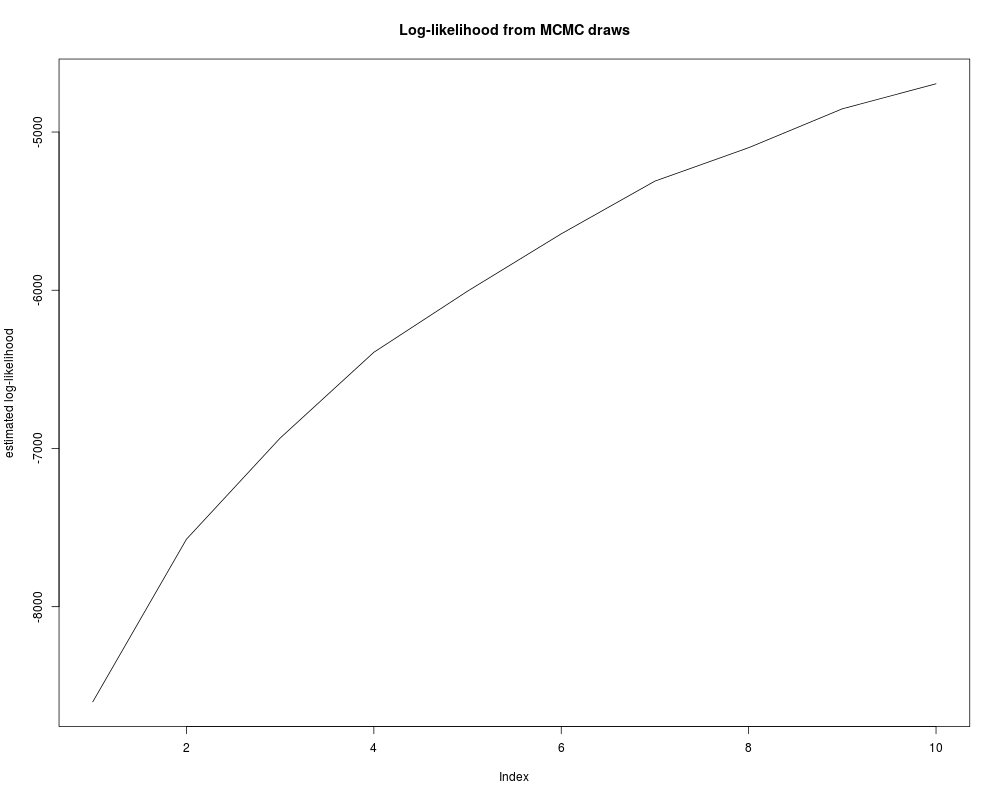
plotLikelihood(random.fit)
intercept = getIntercept(random.fit)
dim(intercept) ##is an array of dimension niter by 15
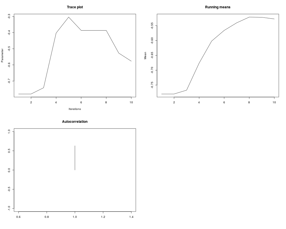
plotDiagnostic(intercept[,1])
plotHLSM.LS(random.fit)
plotHLSM.random.fit(random.fit,parameter = 'Beta')
plotHLSM.random.fit(random.fit,parameter = 'Intercept')
##look at the diagnostic plot of intercept for the first school
#fitting with senderCov and receiverCov
YY = lapply(1:4,function(x)ps.advice.mat[[x]])
nn = sapply(1:4,function(x)nrow(YY[[x]]))
Scov = data.frame(array(NA,dim=c(sum(nn),4)))
a=b=0
for(sid in 1:4){
a = b+1
b = b+nn[sid]
Scov[a:b,1]= sid
Scov[a:b,2]= dimnames(YY[[sid]])[[1]]
Scov[a:b,3] = rnorm(nn[sid],0,1)
Scov[a:b,4] = rnorm(nn[sid],0,1)
}
names(Scov)= c('id','Node','X1','X2')
model1 = HLSMfixedEF(Y=YY,senderCov=Scov,receiverCov=Scov,
niter=10,dd=2,tuneIn=FALSE,intervention=0)
model2 = HLSMrandomEF(Y=YY,senderCov=Scov,receiverCov=Scov,
niter=10,dd=2,tuneIn=FALSE,intervention=0)
Results
R version 3.3.1 (2016-06-21) -- "Bug in Your Hair"
Copyright (C) 2016 The R Foundation for Statistical Computing
Platform: x86_64-pc-linux-gnu (64-bit)

R is free software and comes with ABSOLUTELY NO WARRANTY.
You are welcome to redistribute it under certain conditions.
Type 'license()' or 'licence()' for distribution details.

R is a collaborative project with many contributors.
Type 'contributors()' for more information and
'citation()' on how to cite R or R packages in publications.

Type 'demo()' for some demos, 'help()' for on-line help, or
'help.start()' for an HTML browser interface to help.
Type 'q()' to quit R.

> library(HLSM)
> png(filename="/home/ddbj/snapshot/RGM3/R_CC/result/HLSM/plots.Rd_%03d_medium.png", width=480, height=480)
> ### Name: plotDiagnostic
> ### Title: built-in plot functions for HLSM object
> ### Aliases: plotDiagnostic plotLikelihood plotHLSM.random.fit
> ###   plotHLSM.fixed.fit plotHLSM.LS
>
> ### ** Examples
>
> #using advice seeking network of teachers in 15 schools
> #to fit the data
>
> #Random effect model#
> priors = NULL
> tune = NULL
> initialVals = NULL
> niter = 10
>
> random.fit = HLSMrandomEF(Y = ps.advice.mat,FullX = ps.edge.vars.mat,
+ 	initialVals = initialVals,priors = priors,
+ 	tune = tune,tuneIn = FALSE,dd = 2,niter = niter,
+ 	intervention = 0)
[1] "Starting Values Set"
>
> plotLikelihood(random.fit)
>
> intercept = getIntercept(random.fit)
> dim(intercept) ##is an array of dimension niter by 15
[1] 10 15
> plotDiagnostic(intercept[,1])
> plotHLSM.LS(random.fit)
Error in dev.new(height = 10, width = 10) :
  no suitable unused file name for pdf()
Calls: plotHLSM.LS -> dev.new
Execution halted
 .
.