R Graphical Manual

Browse All

Last data update: 2014.03.03

R: Setting an initial HMM object

hmmsetcont

R Documentation

Setting an initial HMM object

Description

The function sets an initial Hidden Markov Model object with initial set of model parameters. It returns the object of class ContObservHMM that can be analysed with Baum-Welch (function baumwelchcont) and Viterbi algorithms (viterbicont).

Usage

hmmsetcont(Observations, Pi1 = 0.5, Pi2 = 0.5, A11 = 0.7, A12 = 0.3, 
A21 = 0.3, A22 = 0.7, Mu1 = 5, Mu2 = (-5), Var1 = 10, Var2 = 10)

## S3 method for class 'ContObservHMM'
print(x, ...)
## S3 method for class 'ContObservHMM'
summary(object, ...)
## S3 method for class 'ContObservHMM'
plot(x, Series=x$Observations, 
ylabel="Observation series", xlabel="Time", ...)

Arguments

`Observations`	Vector of observations (class "numeric"), a weakly stationary process (e.g. returns time series).
`Pi1`	Initial probability of state 1.
`Pi2`	Initial probability of state 2.
`A11`	Initial transition probability from state 1 to state 1.
`A12`	Initial transition probability from state 1 to state 2.
`A21`	Initial transition probability from state 2 to state 1.
`A22`	Initial transition probability from state 2 to state 2.
`Mu1`	Initial mean for Gaussian PDF for state 1.
`Mu2`	Initial mean for Gaussian PDF for state 2.
`Var1`	Initial variance for Gaussian PDF for state 1.
`Var2`	Initial variance for Gaussian PDF for state 2.
`x`	An object returned by the function `hmmsetcont`.
`object`	An object returned by the function `hmmsetcont`.
`Series`	Observations time series to be plotted along the Markov states.
`ylabel`	Y axis label.
`xlabel`	X axis label.
`...`	Not used.

Value

The function returns an object of the class ContObservHMM that is a list comprising the observations, tables accumulating the model parameters and results after each Baum-Welch iterations (i.e. after each execution of the function baumwelchcont), table for the state sequence derived by the Viterbi algorithm (function viterbicont), and table of the b-probabilities. The object can be analysed with the class-specific functions print, summary, and plot.

Author(s)

Mikhail A. Beketov

Examples


Returns<-logreturns(Prices) # Getting a stationary process
Returns<-Returns*10 		# Scaling the values

hmm<-hmmsetcont(Returns) 	# Creating a HMM object
print(hmm) 					# Checking the initial parameters

for(i in 1:6){hmm<-baumwelchcont(hmm)} # Baum-Welch is 
# executed 6 times and results are accumulated
hmmcomplete<-viterbicont(hmm) # Viterbi execution
print(hmm) 		# Checking the accumulated parameters
summary(hmm) 	# Getting more detailed information
par(mfrow=c(2,1))
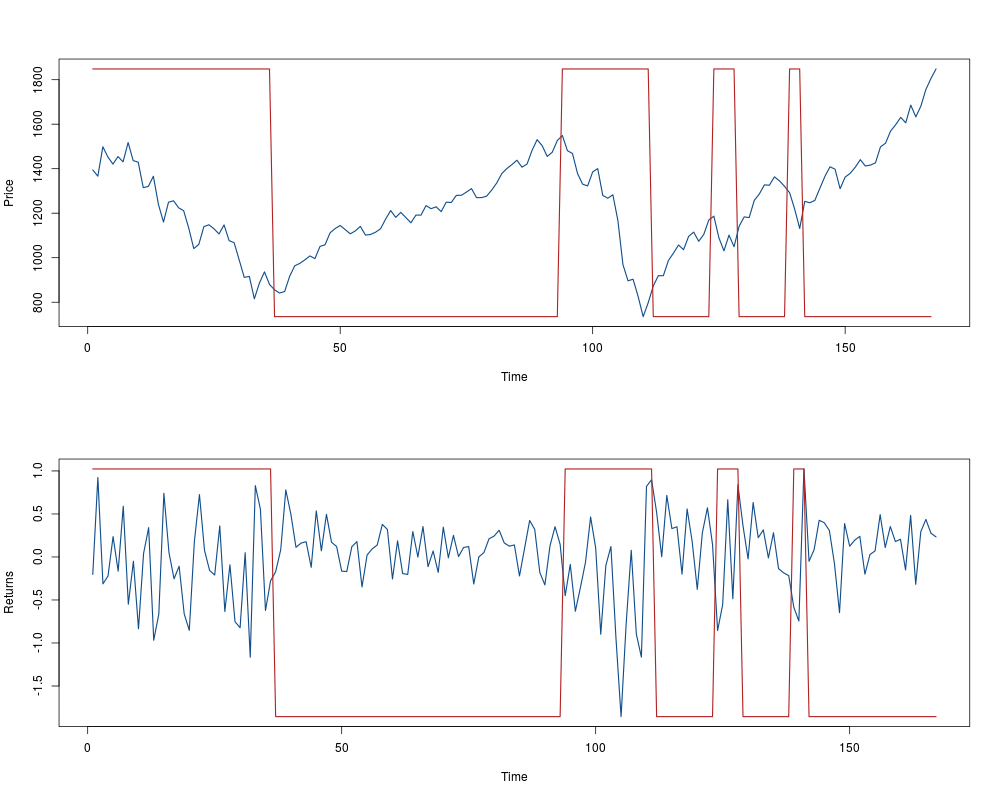
plot(hmmcomplete, Prices, ylabel="Price") 
plot(hmmcomplete, ylabel="Returns") # the revealed 
# Markov chain and the observations are plotted

Results


R version 3.3.1 (2016-06-21) -- "Bug in Your Hair"
Copyright (C) 2016 The R Foundation for Statistical Computing
Platform: x86_64-pc-linux-gnu (64-bit)

R is free software and comes with ABSOLUTELY NO WARRANTY.
You are welcome to redistribute it under certain conditions.
Type 'license()' or 'licence()' for distribution details.

R is a collaborative project with many contributors.
Type 'contributors()' for more information and
'citation()' on how to cite R or R packages in publications.

Type 'demo()' for some demos, 'help()' for on-line help, or
'help.start()' for an HTML browser interface to help.
Type 'q()' to quit R.

> library(HMMCont)
> png(filename="/home/ddbj/snapshot/RGM3/R_CC/result/HMMCont/hmmsetcont.Rd_%03d_medium.png", width=480, height=480)
> ### Name: hmmsetcont
> ### Title: Setting an initial HMM object
> ### Aliases: hmmsetcont print.ContObservHMM summary.ContObservHMM
> ###   plot.ContObservHMM
> ### Keywords: Hidden Markov Model Time series
> 
> ### ** Examples
> 
> 
> Returns<-logreturns(Prices) # Getting a stationary process
> Returns<-Returns*10 		# Scaling the values
> 
> hmm<-hmmsetcont(Returns) 	# Creating a HMM object
> print(hmm) 					# Checking the initial parameters

The number of Baum-Welch iterations: 0
The parameters accumulated so far: 
     Pi1 Pi2 A11 A12 A21 A22 Mu1 Mu2 Var1 Var2
[1,] 0.5 0.5 0.7 0.3 0.3 0.7   5  -5   10   10

The results accumulated so far: 
     P AIC SBIC

The Viterbi algorithm was not yet executed

> 
> for(i in 1:6){hmm<-baumwelchcont(hmm)} # Baum-Welch is 
> # executed 6 times and results are accumulated
> hmmcomplete<-viterbicont(hmm) # Viterbi execution
> print(hmm) 		# Checking the accumulated parameters

The number of Baum-Welch iterations: 6
The parameters accumulated so far: 
      Pi1  Pi2  A11  A12  A21  A22  Mu1   Mu2  Var1  Var2
[1,] 0.50 0.50 0.70 0.30 0.30 0.70 5.00 -5.00 10.00 10.00
[2,] 0.52 0.48 0.71 0.29 0.31 0.69 0.12 -0.09  0.16  0.24
[3,] 0.52 0.48 0.73 0.27 0.31 0.69 0.13 -0.12  0.12  0.28
[4,] 0.48 0.52 0.77 0.23 0.30 0.70 0.14 -0.15  0.10  0.31
[5,] 0.37 0.63 0.81 0.19 0.28 0.72 0.14 -0.17  0.08  0.33
[6,] 0.21 0.79 0.84 0.16 0.25 0.75 0.14 -0.18  0.07  0.35
[7,] 0.08 0.92 0.87 0.13 0.22 0.78 0.14 -0.17  0.07  0.36

The results accumulated so far: 
                 P       AIC      SBIC
[1,] 2.717139e-240 1123.2417 1205.6016
[2,]  7.527195e-45  223.1956  305.5555
[3,]  5.698025e-43  214.5421  296.9020
[4,]  2.149158e-41  207.2818  289.6417
[5,]  2.338101e-40  202.5081  284.8680
[6,]  1.225023e-39  199.1957  281.5556

The Viterbi algorithm was not yet executed

> summary(hmm) 	# Getting more detailed information

The number of observations: 167
The mean of observations: 0.01687374
The SD of observations: 0.4567522
The max and min of observations: 1.023066 and -1.856365

The number of Baum-Welch iterations: 6
The Viterbi algorithm was not yet executed

The parameters accumulated so far: 
      Pi1  Pi2  A11  A12  A21  A22  Mu1   Mu2  Var1  Var2
[1,] 0.50 0.50 0.70 0.30 0.30 0.70 5.00 -5.00 10.00 10.00
[2,] 0.52 0.48 0.71 0.29 0.31 0.69 0.12 -0.09  0.16  0.24
[3,] 0.52 0.48 0.73 0.27 0.31 0.69 0.13 -0.12  0.12  0.28
[4,] 0.48 0.52 0.77 0.23 0.30 0.70 0.14 -0.15  0.10  0.31
[5,] 0.37 0.63 0.81 0.19 0.28 0.72 0.14 -0.17  0.08  0.33
[6,] 0.21 0.79 0.84 0.16 0.25 0.75 0.14 -0.18  0.07  0.35
[7,] 0.08 0.92 0.87 0.13 0.22 0.78 0.14 -0.17  0.07  0.36

The results accumulated so far: 
                 P       AIC      SBIC      HQIC
[1,] 2.717139e-240 1123.2417 1205.6016 1135.8969
[2,]  7.527195e-45  223.1956  305.5555  235.8509
[3,]  5.698025e-43  214.5421  296.9020  227.1973
[4,]  2.149158e-41  207.2818  289.6417  219.9371
[5,]  2.338101e-40  202.5081  284.8680  215.1634
[6,]  1.225023e-39  199.1957  281.5556  211.8510

> par(mfrow=c(2,1))
> plot(hmmcomplete, Prices, ylabel="Price") 
> plot(hmmcomplete, ylabel="Returns") # the revealed 
> # Markov chain and the observations are plotted
> 
> 
> 
> 
> 
> dev.off()
null device 
          1 
>