R: Ternary plot with the Hardy-Weinberg acceptance region
HWTernaryPlot
R Documentation
Ternary plot with the Hardy-Weinberg acceptance region
Description
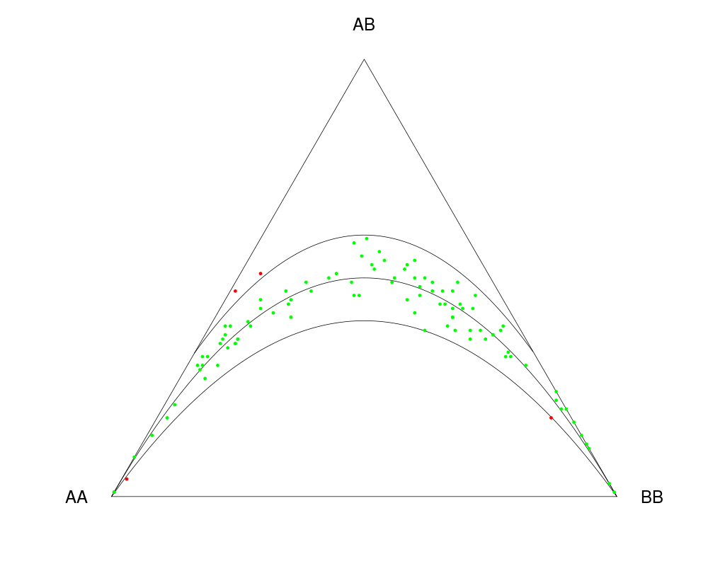
HWTernaryPlot is a routine that draws a ternary plot for three-way genotypic compositions (AA,AB,BB), and represents
the acceptance region for different tests for Hardy-Weinberg equilibrium (HWE) in the plot. This allows for graphical
testing of a large set of markers (e.g. SNPs) for HWE. The (non) significance of the test
for HWE can be inferred from the position of the marker in the ternary plot. Different statistical tests for HWE
can be done graphically with this routine: the ordinary chisquare test, the chisquare test with continuity
correction and the Haldane's exact test.
a matrix of n genotypic compositions or counts. If it
is a matrix of compositions, X should have (n rows that sum
1, and 3 columns, with the relative frequencies of AA, AB and BB
respectively. Argument n should be supplied as well. If X is
a matrix of raw genotypic counts, it should have 3 columns with the
absolute counts of AA, AB and BB respectively. Argument n may
be supplied and will be used for painting acceptance regions. If not
supplied n is computed from the data in X.
n
the samples size (for a complete composition with no missing data).
addmarkers
represent markers by dots in the triangle (addmarkers=TRUE) or not
(addmarkers=FALSE).
newframe
allows for plotting additional markers in an already existing ternary plot. Overplotting
is achieved by setting newframe to FALSE. Setting newframe = TRUE (default) will
create a new ternary plot.
hwcurve
draw the HW parabola in the plot (hwcurve=TRUE) or not (hwcurve=FALSE).
vbounds
indicate the area corresponding to expected counts > 5 (vbounds=TRUE) or not
(vbounds=FALSE).
mafbounds
indicate the area corresponding to MAF < mafvalue.
mafvalue
a critical value for the minor allele frequency (MAF).
axis
draw a vertex axis
0 = no axis is drawn
1 = draw the AA axis
2 = draw the AB axis
3 = draw the BB axis
region
the type of acceptance region to be delimited in the triangle
0 = no acceptance region is drawn
1 = draw the acceptance region corresponding to a Chi-square test
2 = draw the acceptance region corresponding to a Chi-square test with continuity correction
3 = draw the acceptance region corresponding to a Chi-square test with continuity correction for D > 0
4 = draw the acceptance region corresponding to a Chi-square test with continuity correction for D < 0
5 = draw the acceptance regions for all preceding tests simultaneously
6 = draw the acceptance region corresponding to a Chi-square test with continuity correction with the upper
limit for D > 0 and the lower limit for D < 0
7 = draw the acceptance region corresponding to a two-sided exact test
vertexlab
labels for the three vertices of the triangle
alpha
significance level (0.05 by default)
vertex.cex
character expansion factor for the labels of the vertices of the triangle.
pch
the plotting character used to represent the markers.
cc
value for the continuity correction parameter (0.5 by default).
markercol
vector with colours for the marker points in the triangle.
markerbgcol
vector with background colours for the marker points in the triangle.
cex
expansion factor for the marker points in the triangle.
axislab
a label to be put under the horizontal axis.
verbose
print information on the numerically found cut-points between curves of the acceptance region and
the edges of the triangle.
markerlab
labels for the markers in the triangle.
markerpos
positions for the marker labels in the triangle
(1,2,3 or 4).
mcex
character expansion factor for the labels of the markers in the ternary plot.
connect
connect the represented markers by a line in the ternary plot.
curvecols
a vector with four colour specifications for the different curves that can be used
to delimit the HW acceptance region. E.g. curvecols=c("red",
"green","blue","black","purple") will paint
the Hardy-Weinberg curve red, the limits of the acceptance region for an ordinary chi-square test
for HWE green, the limits of the acceptance region for a chi-square test with continuity correction
when D > 0 blue and the limits of the acceptance region for a chi-square test with continuity
correction when D < 0 black, and the limits of the exact acceptance region purple.
signifcolour
colour the marker points automatically according to the result of a signifance test
(green markers non-siginficant, red markers significant).
signifcolour only takes effect if region is set to
1, 2 or 7.
curtyp
style of the drawn curves ("dashed","solid","dotted",...)
ssf
sample size function ("max","min","mean","median",...). Indicates how the sample size for
drawing acceptance regions is determined from the matrix
of counts.
pvaluetype
method to compute p-values in an exact test
("dost" or "selome")
...
other arguments passed on to the plot function (e.g. main for a main title).
Details
HWTernaryPlot automatically colours significant markers in
red, and non-significant markers in green if region is set to
1, 2 or 7.
Value
minp
minimum allele frequency above which testing for HWE is appropriate (expected counts exceeding 5).
maxp
maximum allele frequency below which testing for HWE is appropriate.
inrange
number of markers in the appropriate range.
percinrange
percentage of markers in the appropriate.
nsignif
number of significant markers (only if region equals 1,2 or 7.)
Graffelman, J. and Morales, J. (2008) Graphical Tests for Hardy-Weinberg Equilibrium
Based on the Ternary Plot. Human Heredity 65(2):77-84. http://dx.doi.org/10.1159/000108939.
Graffelman, J. (2015) Exploring Diallelic Genetic Markers: The HardyWeinberg Package.
Journal of Statistical Software 64(3): 1-23. http://www.jstatsoft.org/v64/i03/.
See Also
HWChisq
Examples
n <- 100 # sample size
m <- 100 # number of markers

X <- HWData(n,m)
HWTernaryPlot(X,100,region=1,hwcurve=TRUE,vbounds=FALSE,vertex.cex=2)
Results
R version 3.3.1 (2016-06-21) -- "Bug in Your Hair"
Copyright (C) 2016 The R Foundation for Statistical Computing
Platform: x86_64-pc-linux-gnu (64-bit)

R is free software and comes with ABSOLUTELY NO WARRANTY.
You are welcome to redistribute it under certain conditions.
Type 'license()' or 'licence()' for distribution details.

R is a collaborative project with many contributors.
Type 'contributors()' for more information and
'citation()' on how to cite R or R packages in publications.

Type 'demo()' for some demos, 'help()' for on-line help, or
'help.start()' for an HTML browser interface to help.
Type 'q()' to quit R.

> library(HardyWeinberg)
Loading required package: mice
Loading required package: Rcpp
mice 2.25 2015-11-09
> png(filename="/home/ddbj/snapshot/RGM3/R_CC/result/HardyWeinberg/HWTernaryPlot.Rd_%03d_medium.png", width=480, height=480)
> ### Name: HWTernaryPlot
> ### Title: Ternary plot with the Hardy-Weinberg acceptance region
> ### Aliases: HWTernaryPlot
> ### Keywords: aplot
>
> ### ** Examples
>
>
> n <- 100 # sample size
> m <- 100 # number of markers
>
> X <- HWData(n,m)
> HWTernaryPlot(X,100,region=1,hwcurve=TRUE,vbounds=FALSE,vertex.cex=2)
$minp
[1] 0.2236068

$maxp
[1] 0.7763932

$inrange
[1] 61

$percinrange
[1] 61

$nsignif
[1] 2

>
>
>
>
>
> dev.off()
null device
          1
>
 .
.