How to Hide An Axis in a Hive Plot, with Bonus 2 Plots on One Page

Description

From time-to-time is useful to compare several hive plots based on related data (and you might wish to plot them side-by-side to facilitate comparison). Depending the nature of the data set and how it changes under the experimental design, some data sets may not have any nodes on a particular axis (and therefore, they don't participate in edges either). Let's say your system fundamentally has three axes, but in some data sets one of the axes has no nodes. When you plot them side-by-side, for visual comparison it is nice if all the plots, including the one with an empty axis, have the same general orientation. In other words, even if the data only requires two axes, you might want it plotted as if it had three axes for consistency in overall appearance.

When an axis is present but doesn't have a node on it, this makes plotHive unhappy, but there is a simple solution. You simply put a dummy or phantom node on the empty axis. This is illustrated in the example below. Also demonstrated is a simple grid-based function for putting more than one plot on a device.

Author(s)

Bryan A. Hanson, DePauw University. hanson@depauw.edu

References

http://academic.depauw.edu/~hanson/HiveR/HiveR.html

Examples

require("grid")

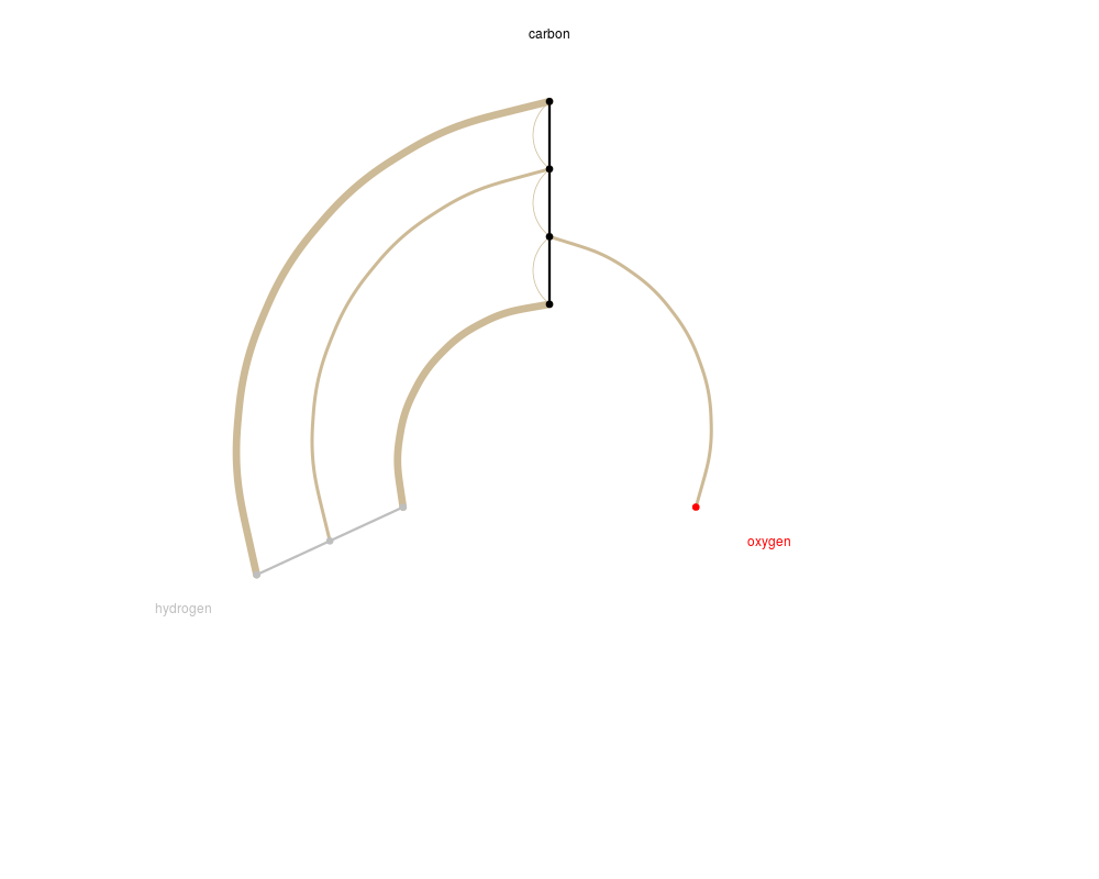
# Adjacency matrix describing the connectivity in 2-butanone
# H's on a single carbon collapsed into a group.
# Matrix entry is bond order.  CH3 is coded so the 
# bond order between C & H is 3 (3 single C-H bonds)

dnames <- c("C1", "C2", "C3", "C4", "O", "HC1", "HC3", "HC4")

#                    C1, C2, C3, C4, O, HC1, HC3, HC4
butanone <- matrix(c( 0,  1,  0,  0, 0,   3,   0,   0, # C1
                      1,  0,  1,  0, 2,   0,   0,   0, # C2
                      0,  1,  0,  1, 0,   0,   2,   0, # C3
                      0,  0,  1,  0, 0,   0,   0,   3, # C4
                      0,  2,  0,  0, 0,   0,   0,   0, # O
                      3,  0,  0,  0, 0,   0,   0,   0, # HC1
                      0,  0,  2,  0, 0,   0,   0,   0, # HC3
                      0,  0,  0,  3, 0,   0,   0,   0), # HC4
             ncol = 8, byrow = TRUE,
             dimnames = list(dnames, dnames))
             
butanoneHPD <- adj2HPD(M = butanone, axis.col = c("black", "gray", "red"),
	desc = "2-butanone")

# Fix up the nodes manually (carbon is on axis 1)
butanoneHPD$nodes$axis[5] <- 3L # oxygen on axis 3
butanoneHPD$nodes$axis[6:8] <- 2L # hydrogen on axis 2
butanoneHPD$nodes$color[5] <- "red"
butanoneHPD$nodes$color[6:8] <- "gray"

# Exaggerate the edge weights, which are proportional to the number of bonds
butanoneHPD$edges$weight <- butanoneHPD$edges$weight^2
butanoneHPD$edges$color <- rep("wheat3", 7)

plotHive(butanoneHPD, method = "rank", bkgnd = "white",
	axLabs = c("carbon", "hydrogen", "oxygen"),
	axLab.pos = c(1, 1, 1), axLab.gpar =
	gpar(col = c("black", "gray", "red")))

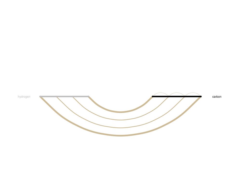
# Now repeat the process for butane

dnames <- c("C1", "C2", "C3", "C4", "HC1", "HC2", "HC3", "HC4")

#                  C1, C2, C3, C4, HC1, HC2, HC3, HC4
butane <- matrix(c( 0,  1,  0,  0,   3,   0,   0,   0, # C1
                    1,  0,  1,  0,   0,   2,   0,   0, # C2
                    0,  1,  0,  1,   0,   0,   2,   0, # C3
                    0,  0,  1,  0,   0,   0,   0,   3, # C4
                    3,  0,  0,  0,   0,   0,   0,   0, # HC1
                    0,  2,  0,  0,   0,   0,   0,   0, # HC2
                    0,  0,  2,  0,   0,   0,   0,   0, # HC3
                    0,  0,  0,  3,   0,   0,   0,   0), # HC4
             ncol = 8, byrow = TRUE,
             dimnames = list(dnames, dnames))
             
butaneHPD <- adj2HPD(M = butane, axis.col = c("black", "gray"),
	desc = "butane")
butaneHPD$nodes$axis[5:8] <- 2L # hydrogen on axis 2
butaneHPD$nodes$color[5:8] <- "gray"
butaneHPD$edges$weight <- butaneHPD$edges$weight^2
butaneHPD$edges$color <- rep("wheat3", 7)

plotHive(butaneHPD, method = "rank", bkgnd = "white",
	axLabs = c("carbon", "hydrogen"),
	axLab.pos = c(1, 1), axLab.gpar = gpar(col = c("black", "gray")))

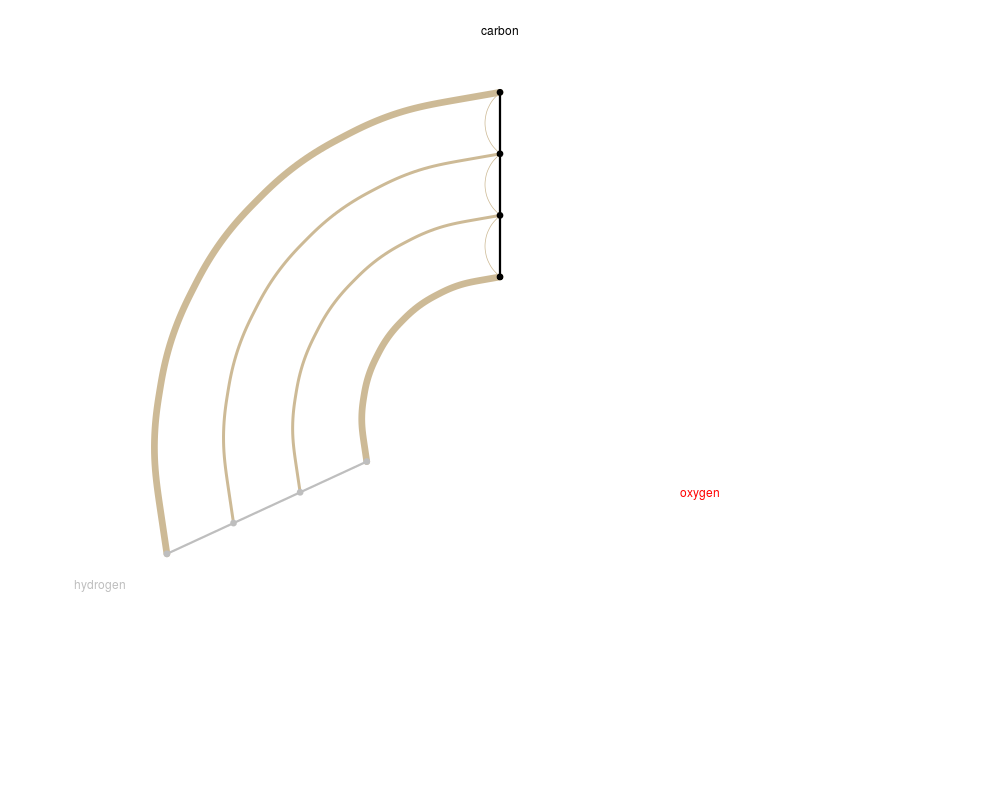
# butaneHPD has 2 axes.  If we wanted to compare to butanoneHPD effectively
# we should add a third dummy axis where the oxygen axis was in butanone
# You might want to look at str(butaneHPD) before beginning

dummy <- c(9, "dummy", 3, 1.0, 1.0, "white") # mixed data types
# but coerced to character
butaneHPD$nodes <- rbind(butaneHPD$nodes, dummy)
str(butaneHPD$nodes) # The data types are mangled from the rbind!

# Now coerce the data types to the standard of the class, and check it
butaneHPD$nodes$id <- as.integer(butaneHPD$nodes$id)
butaneHPD$nodes$axis <- as.integer(butaneHPD$nodes$axis)
butaneHPD$nodes$radius <- as.numeric(butaneHPD$nodes$radius)
butaneHPD$nodes$size <- as.numeric(butaneHPD$nodes$size)
str(butaneHPD$nodes)

chkHPD(butaneHPD) # OK! (False means there were no problems)
sumHPD(butaneHPD)

# Plot it

plotHive(butaneHPD, method = "rank", bkgnd = "white",
	axLabs = c("carbon", "hydrogen", "oxygen"),
	axLab.pos = c(1, 1, 1), axLab.gpar =
	gpar(col = c("black", "gray", "red")))

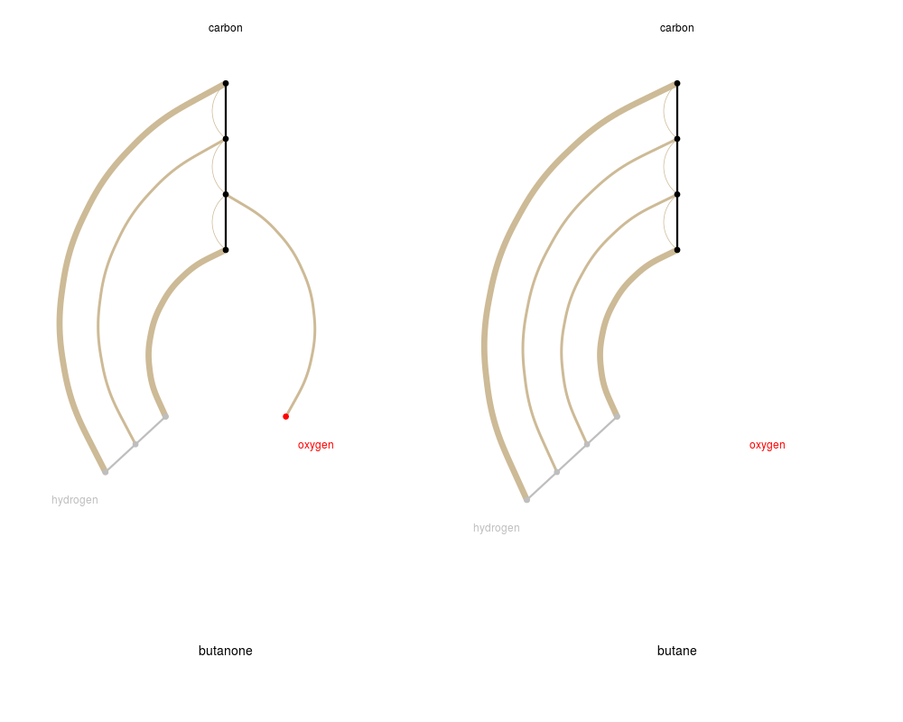
# Put 2 plots side-by-side using a little helper function

vplayout <- function(x, y) viewport(layout.pos.row = x, layout.pos.col = y)

# pdf("Demo.pdf", width = 10, height = 5) # Aspect ratio better
# default screen device

grid.newpage()
pushViewport(viewport(layout = grid.layout(1, 2)))
pushViewport(vplayout(1, 1)) # left plot

plotHive(butanoneHPD, method = "rank", bkgnd = "white",
	axLabs = c("carbon", "hydrogen", "oxygen"),
	axLab.pos = c(1, 1, 1), axLab.gpar =
	gpar(col = c("black", "gray", "red")), np = FALSE)
grid.text("butanone", x = 0.5, y = 0.1, default.units = "npc",
	gp = gpar(fontsize = 14, col = "black"))

popViewport(2)
pushViewport(vplayout(1, 2)) # right plot
grid.text("test2")

plotHive(butaneHPD, method = "rank", bkgnd = "white",
	axLabs = c("carbon", "hydrogen", "oxygen"),
	axLab.pos = c(1, 1, 1), axLab.gpar =
	gpar(col = c("black", "gray", "red")), np = FALSE)
grid.text("butane", x = 0.5, y = 0.1, default.units = "npc",
	gp = gpar(fontsize = 14, col = "black"))

# dev.off()

Results

R version 3.3.1 (2016-06-21) -- "Bug in Your Hair"
Copyright (C) 2016 The R Foundation for Statistical Computing
Platform: x86_64-pc-linux-gnu (64-bit)

R is free software and comes with ABSOLUTELY NO WARRANTY.
You are welcome to redistribute it under certain conditions.
Type 'license()' or 'licence()' for distribution details.

R is a collaborative project with many contributors.
Type 'contributors()' for more information and
'citation()' on how to cite R or R packages in publications.

Type 'demo()' for some demos, 'help()' for on-line help, or
'help.start()' for an HTML browser interface to help.
Type 'q()' to quit R.

> library(HiveR)
> png(filename="/home/ddbj/snapshot/RGM3/R_CC/result/HiveR/HidingAnAxis.Rd_%03d_medium.png", width=480, height=480)
> ### Name: HidingAnAxis
> ### Title: How to Hide An Axis in a Hive Plot, with Bonus 2 Plots on One
> ###   Page
> ### Aliases: HidingAnAxis TwoPlotsOnePage
> 
> ### ** Examples
> 
> require("grid")
Loading required package: grid
> 
> # Adjacency matrix describing the connectivity in 2-butanone
> # H's on a single carbon collapsed into a group.
> # Matrix entry is bond order.  CH3 is coded so the 
> # bond order between C & H is 3 (3 single C-H bonds)
> 
> dnames <- c("C1", "C2", "C3", "C4", "O", "HC1", "HC3", "HC4")
> 
> #                    C1, C2, C3, C4, O, HC1, HC3, HC4
> butanone <- matrix(c( 0,  1,  0,  0, 0,   3,   0,   0, # C1
+                       1,  0,  1,  0, 2,   0,   0,   0, # C2
+                       0,  1,  0,  1, 0,   0,   2,   0, # C3
+                       0,  0,  1,  0, 0,   0,   0,   3, # C4
+                       0,  2,  0,  0, 0,   0,   0,   0, # O
+                       3,  0,  0,  0, 0,   0,   0,   0, # HC1
+                       0,  0,  2,  0, 0,   0,   0,   0, # HC3
+                       0,  0,  0,  3, 0,   0,   0,   0), # HC4
+              ncol = 8, byrow = TRUE,
+              dimnames = list(dnames, dnames))
>              
> butanoneHPD <- adj2HPD(M = butanone, axis.col = c("black", "gray", "red"),
+ 	desc = "2-butanone")
Matrix is symmetric, using only the lower triangle
> 
> # Fix up the nodes manually (carbon is on axis 1)
> butanoneHPD$nodes$axis[5] <- 3L # oxygen on axis 3
> butanoneHPD$nodes$axis[6:8] <- 2L # hydrogen on axis 2
> butanoneHPD$nodes$color[5] <- "red"
> butanoneHPD$nodes$color[6:8] <- "gray"
> 
> # Exaggerate the edge weights, which are proportional to the number of bonds
> butanoneHPD$edges$weight <- butanoneHPD$edges$weight^2
> butanoneHPD$edges$color <- rep("wheat3", 7)
> 
> plotHive(butanoneHPD, method = "rank", bkgnd = "white",
+ 	axLabs = c("carbon", "hydrogen", "oxygen"),
+ 	axLab.pos = c(1, 1, 1), axLab.gpar =
+ 	gpar(col = c("black", "gray", "red")))
> 
> # Now repeat the process for butane
> 
> dnames <- c("C1", "C2", "C3", "C4", "HC1", "HC2", "HC3", "HC4")
> 
> #                  C1, C2, C3, C4, HC1, HC2, HC3, HC4
> butane <- matrix(c( 0,  1,  0,  0,   3,   0,   0,   0, # C1
+                     1,  0,  1,  0,   0,   2,   0,   0, # C2
+                     0,  1,  0,  1,   0,   0,   2,   0, # C3
+                     0,  0,  1,  0,   0,   0,   0,   3, # C4
+                     3,  0,  0,  0,   0,   0,   0,   0, # HC1
+                     0,  2,  0,  0,   0,   0,   0,   0, # HC2
+                     0,  0,  2,  0,   0,   0,   0,   0, # HC3
+                     0,  0,  0,  3,   0,   0,   0,   0), # HC4
+              ncol = 8, byrow = TRUE,
+              dimnames = list(dnames, dnames))
>              
> butaneHPD <- adj2HPD(M = butane, axis.col = c("black", "gray"),
+ 	desc = "butane")
Matrix is symmetric, using only the lower triangle
> butaneHPD$nodes$axis[5:8] <- 2L # hydrogen on axis 2
> butaneHPD$nodes$color[5:8] <- "gray"
> butaneHPD$edges$weight <- butaneHPD$edges$weight^2
> butaneHPD$edges$color <- rep("wheat3", 7)
> 
> plotHive(butaneHPD, method = "rank", bkgnd = "white",
+ 	axLabs = c("carbon", "hydrogen"),
+ 	axLab.pos = c(1, 1), axLab.gpar = gpar(col = c("black", "gray")))
> 
> # butaneHPD has 2 axes.  If we wanted to compare to butanoneHPD effectively
> # we should add a third dummy axis where the oxygen axis was in butanone
> # You might want to look at str(butaneHPD) before beginning
> 
> dummy <- c(9, "dummy", 3, 1.0, 1.0, "white") # mixed data types
> # but coerced to character
> butaneHPD$nodes <- rbind(butaneHPD$nodes, dummy)
> str(butaneHPD$nodes) # The data types are mangled from the rbind!
'data.frame':	9 obs. of  6 variables:
 $ id    : chr  "1" "2" "3" "4" ...
 $ lab   : chr  "C1" "C2" "C3" "C4" ...
 $ axis  : chr  "1" "1" "1" "1" ...
 $ radius: chr  "1" "1" "1" "1" ...
 $ size  : chr  "1" "1" "1" "1" ...
 $ color : chr  "black" "black" "black" "black" ...
> 
> # Now coerce the data types to the standard of the class, and check it
> butaneHPD$nodes$id <- as.integer(butaneHPD$nodes$id)
> butaneHPD$nodes$axis <- as.integer(butaneHPD$nodes$axis)
> butaneHPD$nodes$radius <- as.numeric(butaneHPD$nodes$radius)
> butaneHPD$nodes$size <- as.numeric(butaneHPD$nodes$size)
> str(butaneHPD$nodes)
'data.frame':	9 obs. of  6 variables:
 $ id    : int  1 2 3 4 5 6 7 8 9
 $ lab   : chr  "C1" "C2" "C3" "C4" ...
 $ axis  : int  1 1 1 1 2 2 2 2 3
 $ radius: num  1 1 1 1 1 1 1 1 1
 $ size  : num  1 1 1 1 1 1 1 1 1
 $ color : chr  "black" "black" "black" "black" ...
> 
> chkHPD(butaneHPD) # OK! (False means there were no problems)
[1] FALSE
> sumHPD(butaneHPD)
	butane
	This hive plot data set contains 9 nodes on 3 axes and 7 edges.
	It is a  2D data set.

		Axis 1 has 4 nodes spanning radii from 1 to 1 
		Axis 2 has 4 nodes spanning radii from 1 to 1 
		Axis 3 has 1 nodes spanning radii from 1 to 1 

		Axes 1 and 1 share 3 edges
		Axes 2 and 1 share 4 edges

> 
> # Plot it
> 
> plotHive(butaneHPD, method = "rank", bkgnd = "white",
+ 	axLabs = c("carbon", "hydrogen", "oxygen"),
+ 	axLab.pos = c(1, 1, 1), axLab.gpar =
+ 	gpar(col = c("black", "gray", "red")))
> 
> # Put 2 plots side-by-side using a little helper function
> 
> vplayout <- function(x, y) viewport(layout.pos.row = x, layout.pos.col = y)
> 
> # pdf("Demo.pdf", width = 10, height = 5) # Aspect ratio better
> # default screen device
> 
> grid.newpage()
> pushViewport(viewport(layout = grid.layout(1, 2)))
> pushViewport(vplayout(1, 1)) # left plot
> 
> plotHive(butanoneHPD, method = "rank", bkgnd = "white",
+ 	axLabs = c("carbon", "hydrogen", "oxygen"),
+ 	axLab.pos = c(1, 1, 1), axLab.gpar =
+ 	gpar(col = c("black", "gray", "red")), np = FALSE)
> grid.text("butanone", x = 0.5, y = 0.1, default.units = "npc",
+ 	gp = gpar(fontsize = 14, col = "black"))
> 
> popViewport(2)
> pushViewport(vplayout(1, 2)) # right plot
> grid.text("test2")
> 
> plotHive(butaneHPD, method = "rank", bkgnd = "white",
+ 	axLabs = c("carbon", "hydrogen", "oxygen"),
+ 	axLab.pos = c(1, 1, 1), axLab.gpar =
+ 	gpar(col = c("black", "gray", "red")), np = FALSE)
> grid.text("butane", x = 0.5, y = 0.1, default.units = "npc",
+ 	gp = gpar(fontsize = 14, col = "black"))
> 
> # dev.off()
> 
> 
> 
> 
> 
> dev.off()
null device 
          1 
>