Additive Regression with Optimal Transformations on Both Sides using Canonical Variates

Description

Expands continuous variables into restricted cubic spline bases and categorical variables into dummy variables and fits a multivariate equation using canonical variates. This finds optimum transformations that maximize R^2. Optionally, the bootstrap is used to estimate the covariance matrix of both left- and right-hand-side transformation parameters, and to estimate the bias in the R^2 due to overfitting and compute the bootstrap optimism-corrected R^2. Cross-validation can also be used to get an unbiased estimate of R^2 but this is not as precise as the bootstrap estimate. The bootstrap and cross-validation may also used to get estimates of mean and median absolute error in predicted values on the original y scale. These two estimates are perhaps the best ones for gauging the accuracy of a flexible model, because it is difficult to compare R^2 under different y-transformations, and because R^2 allows for an out-of-sample recalibration (i.e., it only measures relative errors).

Note that uncertainty about the proper transformation of y causes an enormous amount of model uncertainty. When the transformation for y is estimated from the data a high variance in predicted values on the original y scale may result, especially if the true transformation is linear. Comparing bootstrap or cross-validated mean absolute errors with and without restricted the y transform to be linear (ytype='l') may help the analyst choose the proper model complexity.

Usage

areg(x, y, xtype = NULL, ytype = NULL, nk = 4,
     B = 0, na.rm = TRUE, tolerance = NULL, crossval = NULL)

## S3 method for class 'areg'
print(x, digits=4, ...)

## S3 method for class 'areg'
plot(x, whichx = 1:ncol(x$x), ...)

## S3 method for class 'areg'
predict(object, x, type=c('lp','fitted','x'),
                       what=c('all','sample'), ...)

Arguments

Details

areg is a competitor of ace in the acepack package. Transformations from ace are seldom smooth enough and are often overfitted. With areg the complexity can be controlled with the nk parameter, and predicted values are easy to obtain because parametric functions are fitted.

If one side of the equation has a categorical variable with more than two categories and the other side has a continuous variable not assumed to act linearly, larger sample sizes are needed to reliably estimate transformations, as it is difficult to optimally score categorical variables to maximize R^2 against a simultaneously optimally transformed continuous variable.

Value

a list of class "areg" containing many objects

Author(s)

Frank Harrell
Department of Biostatistics
Vanderbilt University
f.harrell@vanderbilt.edu

References

Breiman and Friedman, Journal of the American Statistical Association (September, 1985).

See Also

cancor,ace, transcan

Examples

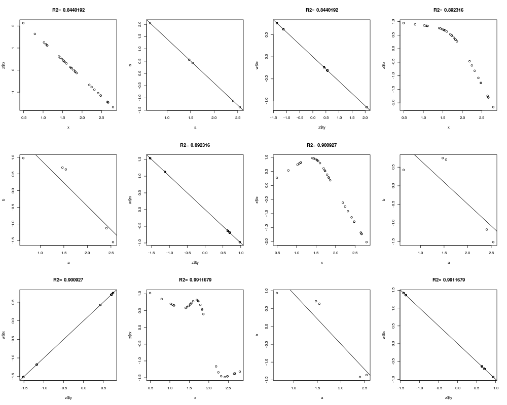
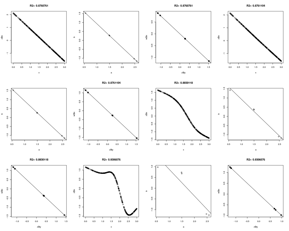
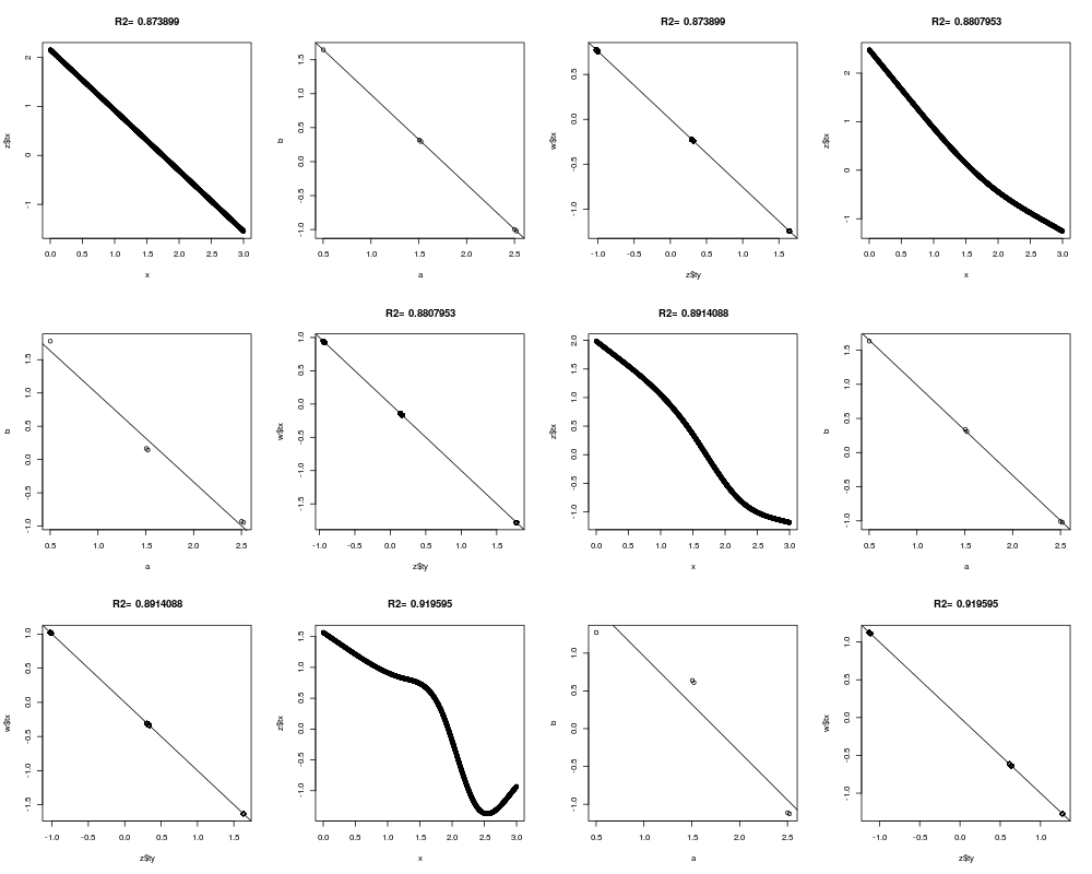
set.seed(1)

ns <- c(30,300,3000)
for(n in ns) {
  y <- sample(1:5, n, TRUE)
  x <- abs(y-3) + runif(n)
  par(mfrow=c(3,4))
  for(k in c(0,3:5)) {
    z <- areg(x, y, ytype='c', nk=k)
    plot(x, z$tx)
	title(paste('R2=',format(z$rsquared)))
    tapply(z$ty, y, range)
    a <- tapply(x,y,mean)
    b <- tapply(z$ty,y,mean)
    plot(a,b)
	abline(lsfit(a,b))
    # Should get same result to within linear transformation if reverse x and y
    w <- areg(y, x, xtype='c', nk=k)
    plot(z$ty, w$tx)
    title(paste('R2=',format(w$rsquared)))
    abline(lsfit(z$ty, w$tx))
 }
}

par(mfrow=c(2,2))
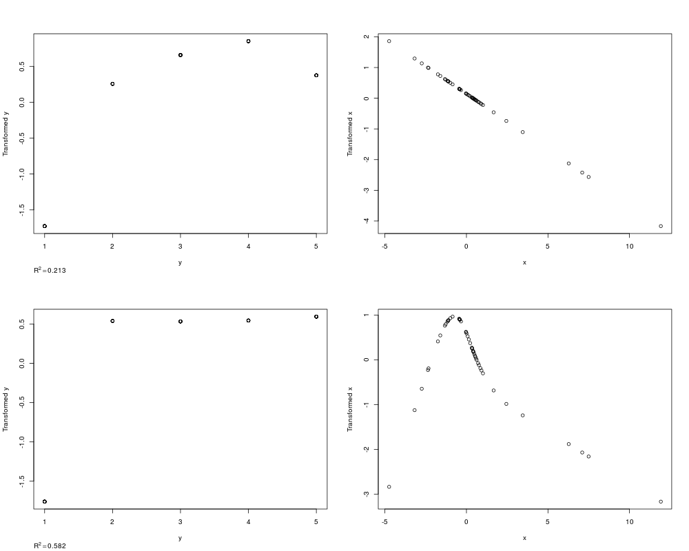
# Example where one category in y differs from others but only in variance of x
n <- 50
y <- sample(1:5,n,TRUE)
x <- rnorm(n)
x[y==1] <- rnorm(sum(y==1), 0, 5)
z <- areg(x,y,xtype='l',ytype='c')
z
plot(z)
z <- areg(x,y,ytype='c')
z
plot(z)

## Not run: 		
# Examine overfitting when true transformations are linear
par(mfrow=c(4,3))
for(n in c(200,2000)) {
  x <- rnorm(n); y <- rnorm(n) + x
    for(nk in c(0,3,5)) {
    z <- areg(x, y, nk=nk, crossval=10, B=100)
    print(z)
    plot(z)
    title(paste('n=',n))
  }
}
par(mfrow=c(1,1))

# Underfitting when true transformation is quadratic but overfitting
# when y is allowed to be transformed
set.seed(49)
n <- 200
x <- rnorm(n); y <- rnorm(n) + .5*x^2
#areg(x, y, nk=0, crossval=10, B=100)
#areg(x, y, nk=4, ytype='l', crossval=10, B=100)
z <- areg(x, y, nk=4) #, crossval=10, B=100)
z
# Plot x vs. predicted value on original scale.  Since y-transform is
# not monotonic, there are multiple y-inverses
xx <- seq(-3.5,3.5,length=1000)
yhat <- predict(z, xx, type='fitted')
plot(x, y, xlim=c(-3.5,3.5))
for(j in 1:ncol(yhat)) lines(xx, yhat[,j], col=j)
# Plot a random sample of possible y inverses
yhats <- predict(z, xx, type='fitted', what='sample')
points(xx, yhats, pch=2)

## End(Not run)

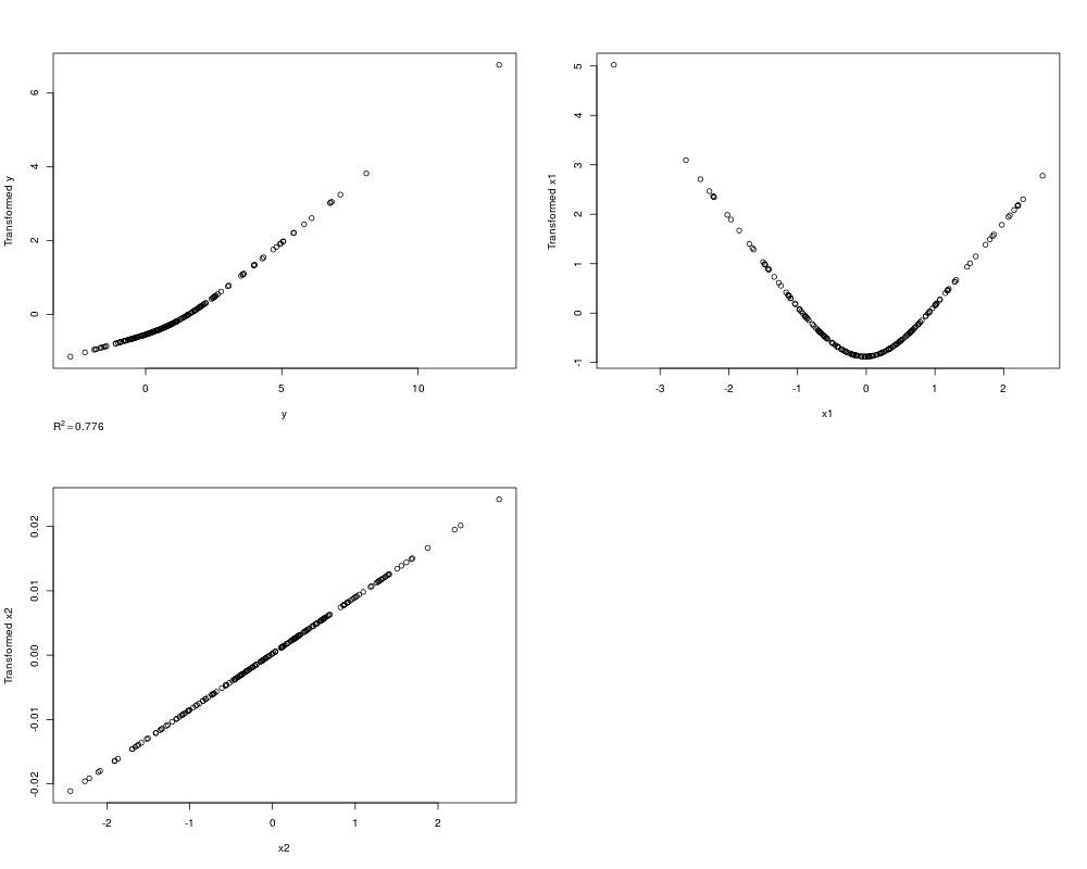
# True transformation of x1 is quadratic, y is linear
n <- 200
x1 <- rnorm(n); x2 <- rnorm(n); y <- rnorm(n) + x1^2
z <- areg(cbind(x1,x2),y,xtype=c('s','l'),nk=3)
par(mfrow=c(2,2))
plot(z)

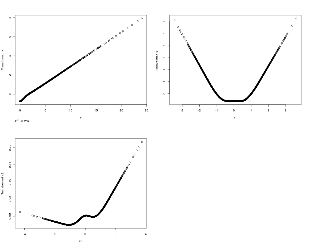
# y transformation is inverse quadratic but areg gets the same answer by
# making x1 quadratic
n <- 5000
x1 <- rnorm(n); x2 <- rnorm(n); y <- (x1 + rnorm(n))^2
z <- areg(cbind(x1,x2),y,nk=5)
par(mfrow=c(2,2))
plot(z)

# Overfit 20 predictors when no true relationships exist
n <- 1000
x <- matrix(runif(n*20),n,20)
y <- rnorm(n)
z <- areg(x, y, nk=5)  # add crossval=4 to expose the problem

# Test predict function
n <- 50
x <- rnorm(n)
y <- rnorm(n) + x
g <- sample(1:3, n, TRUE)
z <- areg(cbind(x,g),y,xtype=c('s','c'))
range(predict(z, cbind(x,g)) - z$linear.predictors)

Results

R version 3.3.1 (2016-06-21) -- "Bug in Your Hair"
Copyright (C) 2016 The R Foundation for Statistical Computing
Platform: x86_64-pc-linux-gnu (64-bit)

R is free software and comes with ABSOLUTELY NO WARRANTY.
You are welcome to redistribute it under certain conditions.
Type 'license()' or 'licence()' for distribution details.

R is a collaborative project with many contributors.
Type 'contributors()' for more information and
'citation()' on how to cite R or R packages in publications.

Type 'demo()' for some demos, 'help()' for on-line help, or
'help.start()' for an HTML browser interface to help.
Type 'q()' to quit R.

> library(Hmisc)
Loading required package: lattice
Loading required package: survival
Loading required package: Formula
Loading required package: ggplot2

Attaching package: 'Hmisc'

The following objects are masked from 'package:base':

    format.pval, round.POSIXt, trunc.POSIXt, units

> png(filename="/home/ddbj/snapshot/RGM3/R_CC/result/Hmisc/areg.Rd_%03d_medium.png", width=480, height=480)
> ### Name: areg
> ### Title: Additive Regression with Optimal Transformations on Both Sides
> ###   using Canonical Variates
> ### Aliases: areg print.areg predict.areg plot.areg
> ### Keywords: smooth regression multivariate models
> 
> ### ** Examples
> 
> set.seed(1)
> 
> ns <- c(30,300,3000)
> for(n in ns) {
+   y <- sample(1:5, n, TRUE)
+   x <- abs(y-3) + runif(n)
+   par(mfrow=c(3,4))
+   for(k in c(0,3:5)) {
+     z <- areg(x, y, ytype='c', nk=k)
+     plot(x, z$tx)
+ 	title(paste('R2=',format(z$rsquared)))
+     tapply(z$ty, y, range)
+     a <- tapply(x,y,mean)
+     b <- tapply(z$ty,y,mean)
+     plot(a,b)
+ 	abline(lsfit(a,b))
+     # Should get same result to within linear transformation if reverse x and y
+     w <- areg(y, x, xtype='c', nk=k)
+     plot(z$ty, w$tx)
+     title(paste('R2=',format(w$rsquared)))
+     abline(lsfit(z$ty, w$tx))
+  }
+ }
> 
> par(mfrow=c(2,2))
> # Example where one category in y differs from others but only in variance of x
> n <- 50
> y <- sample(1:5,n,TRUE)
> x <- rnorm(n)
> x[y==1] <- rnorm(sum(y==1), 0, 5)
> z <- areg(x,y,xtype='l',ytype='c')
> z

N: 50 	 0  observations with NAs deleted.
R^2: 0.213	nk: 4	Mean and Median |error|: 2.06, 2


  type d.f.
x    l    1

y type: c 	d.f.: 4 

> plot(z)
> z <- areg(x,y,ytype='c')
> z

N: 50 	 0  observations with NAs deleted.
R^2: 0.582	nk: 4	Mean and Median |error|: 2.06, 2


  type d.f.
x    s    3

y type: c 	d.f.: 4 

> plot(z)
> 
> ## Not run: 
> ##D 		
> ##D # Examine overfitting when true transformations are linear
> ##D par(mfrow=c(4,3))
> ##D for(n in c(200,2000)) {
> ##D   x <- rnorm(n); y <- rnorm(n) + x
> ##D     for(nk in c(0,3,5)) {
> ##D     z <- areg(x, y, nk=nk, crossval=10, B=100)
> ##D     print(z)
> ##D     plot(z)
> ##D     title(paste('n=',n))
> ##D   }
> ##D }
> ##D par(mfrow=c(1,1))
> ##D 
> ##D # Underfitting when true transformation is quadratic but overfitting
> ##D # when y is allowed to be transformed
> ##D set.seed(49)
> ##D n <- 200
> ##D x <- rnorm(n); y <- rnorm(n) + .5*x^2
> ##D #areg(x, y, nk=0, crossval=10, B=100)
> ##D #areg(x, y, nk=4, ytype='l', crossval=10, B=100)
> ##D z <- areg(x, y, nk=4) #, crossval=10, B=100)
> ##D z
> ##D # Plot x vs. predicted value on original scale.  Since y-transform is
> ##D # not monotonic, there are multiple y-inverses
> ##D xx <- seq(-3.5,3.5,length=1000)
> ##D yhat <- predict(z, xx, type='fitted')
> ##D plot(x, y, xlim=c(-3.5,3.5))
> ##D for(j in 1:ncol(yhat)) lines(xx, yhat[,j], col=j)
> ##D # Plot a random sample of possible y inverses
> ##D yhats <- predict(z, xx, type='fitted', what='sample')
> ##D points(xx, yhats, pch=2)
> ## End(Not run)
> 
> # True transformation of x1 is quadratic, y is linear
> n <- 200
> x1 <- rnorm(n); x2 <- rnorm(n); y <- rnorm(n) + x1^2
> z <- areg(cbind(x1,x2),y,xtype=c('s','l'),nk=3)
> par(mfrow=c(2,2))
> plot(z)
> 
> # y transformation is inverse quadratic but areg gets the same answer by
> # making x1 quadratic
> n <- 5000
> x1 <- rnorm(n); x2 <- rnorm(n); y <- (x1 + rnorm(n))^2
> z <- areg(cbind(x1,x2),y,nk=5)
> par(mfrow=c(2,2))
> plot(z)
> 
> # Overfit 20 predictors when no true relationships exist
> n <- 1000
> x <- matrix(runif(n*20),n,20)
> y <- rnorm(n)
> z <- areg(x, y, nk=5)  # add crossval=4 to expose the problem
> 
> # Test predict function
> n <- 50
> x <- rnorm(n)
> y <- rnorm(n) + x
> g <- sample(1:3, n, TRUE)
> z <- areg(cbind(x,g),y,xtype=c('s','c'))
> range(predict(z, cbind(x,g)) - z$linear.predictors)
[1] 0 0
> 
> 
> 
> 
> 
> dev.off()
null device 
          1 
>