Supported by Dr. Osamu Ogasawara and  . . |
|
Last data update: 2014.03.03 |
Multiple Imputation using Additive Regression, Bootstrapping, and Predictive Mean MatchingDescriptionThe
Instead of defaulting to taking random draws from fitted imputation
models using random residuals as is done by A If a target variable is transformed nonlinearly (i.e., if The Usage
aregImpute(formula, data, subset, n.impute=5, group=NULL,
           nk=3, tlinear=TRUE, type=c('pmm','regression','normpmm'),
           pmmtype=1, match=c('weighted','closest','kclosest'),
           kclosest=3, fweighted=0.2,
           curtail=TRUE, boot.method=c('simple', 'approximate bayesian'),
           burnin=3, x=FALSE, pr=TRUE, plotTrans=FALSE, tolerance=NULL, B=75)
## S3 method for class 'aregImpute'
print(x, digits=3, ...)
## S3 method for class 'aregImpute'
plot(x, nclass=NULL, type=c('ecdf','hist'),
     datadensity=c("hist", "none", "rug", "density"),
     diagnostics=FALSE, maxn=10, ...)
reformM(formula, data, nperm)
Arguments
DetailsThe sequence of steps used by the When When the missingness mechanism for a variable is so systematic that the
distribution of observed values is truncated, predictive mean matching
does not work. It will only yield imputed values that are near observed
values, so intervals in which no values are observed will not be
populated by imputed values. For this case, the only hope is to make
regression assumptions and use extrapolation. With
As model uncertainty is high when the transformation of a target
variable is unknown, Valuea list of class
Author(s)Frank Harrell
Referencesvan Buuren, Stef. Flexible Imputation of Missing Data. Chapman & Hall/CRC, Boca Raton FL, 2012. Little R, An H. Robust likelihood-based analysis of multivariate data with missing values. Statistica Sinica 14:949-968, 2004. van Buuren S, Brand JPL, Groothuis-Oudshoorn CGM, Rubin DB. Fully conditional specifications in multivariate imputation. J Stat Comp Sim 72:1049-1064, 2006. de Groot JAH, Janssen KJM, Zwinderman AH, Moons KGM, Reitsma JB. Multiple imputation to correct for partial verification bias revisited. Stat Med 27:5880-5889, 2008. Siddique J. Multiple imputation using an iterative hot-deck with distance-based donor selection. Stat Med 27:83-102, 2008. White IR, Royston P, Wood AM. Multiple imputation using chained equations: Issues and guidance for practice. Stat Med 30:377-399, 2011. See Also
Examples
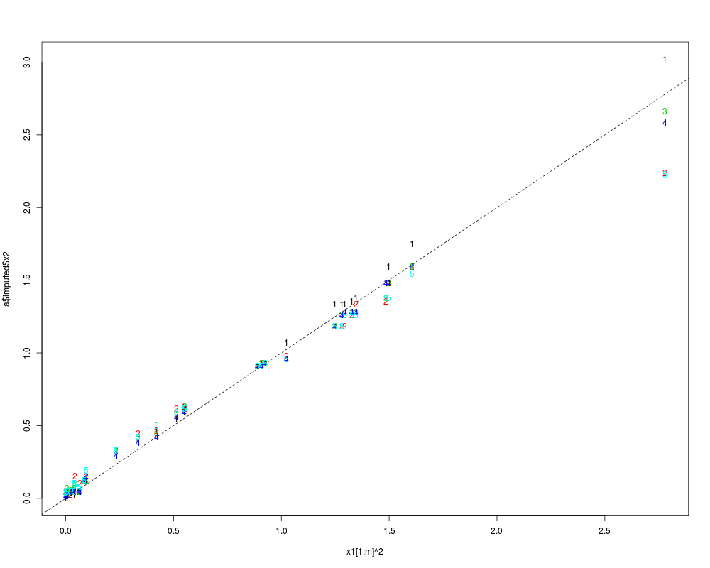
# Check that aregImpute can almost exactly estimate missing values when
# there is a perfect nonlinear relationship between two variables
# Fit restricted cubic splines with 4 knots for x1 and x2, linear for x3
set.seed(3)
x1 <- rnorm(200)
x2 <- x1^2
x3 <- runif(200)
m <- 30
x2[1:m] <- NA
a <- aregImpute(~x1+x2+I(x3), n.impute=5, nk=4, match='closest')
a
matplot(x1[1:m]^2, a$imputed$x2)
abline(a=0, b=1, lty=2)

x1[1:m]^2
a$imputed$x2


# Multiple imputation and estimation of variances and covariances of
# regression coefficient estimates accounting for imputation
# Example 1: large sample size, much missing data, no overlap in
# NAs across variables
x1 <- factor(sample(c('a','b','c'),1000,TRUE))
x2 <- (x1=='b') + 3*(x1=='c') + rnorm(1000,0,2)
x3 <- rnorm(1000)
y  <- x2 + 1*(x1=='c') + .2*x3 + rnorm(1000,0,2)
orig.x1 <- x1[1:250]
orig.x2 <- x2[251:350]
x1[1:250] <- NA
x2[251:350] <- NA
d <- data.frame(x1,x2,x3,y)
# Find value of nk that yields best validating imputation models
# tlinear=FALSE means to not force the target variable to be linear
f <- aregImpute(~y + x1 + x2 + x3, nk=c(0,3:5), tlinear=FALSE,
                data=d, B=10) # normally B=75
f
# Try forcing target variable (x1, then x2) to be linear while allowing
# predictors to be nonlinear (could also say tlinear=TRUE)
f <- aregImpute(~y + x1 + x2 + x3, nk=c(0,3:5), data=d, B=10)
f

## Not run:
# Use 100 imputations to better check against individual true values
f <- aregImpute(~y + x1 + x2 + x3, n.impute=100, data=d)
f
par(mfrow=c(2,1))
plot(f)
modecat <- function(u) {
 tab <- table(u)
 as.numeric(names(tab)[tab==max(tab)][1])
}
table(orig.x1,apply(f$imputed$x1, 1, modecat))
par(mfrow=c(1,1))
plot(orig.x2, apply(f$imputed$x2, 1, mean))
fmi <- fit.mult.impute(y ~ x1 + x2 + x3, lm, f,
                       data=d)
sqrt(diag(vcov(fmi)))
fcc <- lm(y ~ x1 + x2 + x3)
summary(fcc)   # SEs are larger than from mult. imputation

## End(Not run)
## Not run:
# Example 2: Very discriminating imputation models,
# x1 and x2 have some NAs on the same rows, smaller n
set.seed(5)
x1 <- factor(sample(c('a','b','c'),100,TRUE))
x2 <- (x1=='b') + 3*(x1=='c') + rnorm(100,0,.4)
x3 <- rnorm(100)
y  <- x2 + 1*(x1=='c') + .2*x3 + rnorm(100,0,.4)
orig.x1 <- x1[1:20]
orig.x2 <- x2[18:23]
x1[1:20] <- NA
x2[18:23] <- NA
#x2[21:25] <- NA
d <- data.frame(x1,x2,x3,y)
n <- naclus(d)
plot(n); naplot(n)  # Show patterns of NAs
# 100 imputations to study them; normally use 5 or 10
f  <- aregImpute(~y + x1 + x2 + x3, n.impute=100, nk=0, data=d)
par(mfrow=c(2,3))
plot(f, diagnostics=TRUE, maxn=2)
# Note: diagnostics=TRUE makes graphs similar to those made by:
# r <- range(f$imputed$x2, orig.x2)
# for(i in 1:6) {  # use 1:2 to mimic maxn=2
#   plot(1:100, f$imputed$x2[i,], ylim=r,
#        ylab=paste("Imputations for Obs.",i))
#   abline(h=orig.x2[i],lty=2)
# }

table(orig.x1,apply(f$imputed$x1, 1, modecat))
par(mfrow=c(1,1))
plot(orig.x2, apply(f$imputed$x2, 1, mean))


fmi <- fit.mult.impute(y ~ x1 + x2, lm, f,
                       data=d)
sqrt(diag(vcov(fmi)))
fcc <- lm(y ~ x1 + x2)
summary(fcc)   # SEs are larger than from mult. imputation

## End(Not run)

## Not run:
# Study relationship between smoothing parameter for weighting function
# (multiplier of mean absolute distance of transformed predicted
# values, used in tricube weighting function) and standard deviation
# of multiple imputations.  SDs are computed from average variances
# across subjects.  match="closest" same as match="weighted" with
# small value of fweighted.
# This example also shows problems with predicted mean
# matching almost always giving the same imputed values when there is
# only one predictor (regression coefficients change over multiple
# imputations but predicted values are virtually 1-1 functions of each
# other)

set.seed(23)
x <- runif(200)
y <- x + runif(200, -.05, .05)
r <- resid(lsfit(x,y))
rmse <- sqrt(sum(r^2)/(200-2))   # sqrt of residual MSE

y[1:20] <- NA
d <- data.frame(x,y)
f <- aregImpute(~ x + y, n.impute=10, match='closest', data=d)
# As an aside here is how to create a completed dataset for imputation
# number 3 as fit.mult.impute would do automatically.  In this degenerate
# case changing 3 to 1-2,4-10 will not alter the results.
imputed <- impute.transcan(f, imputation=3, data=d, list.out=TRUE,
                           pr=FALSE, check=FALSE)
sd <- sqrt(mean(apply(f$imputed$y, 1, var)))

ss <- c(0, .01, .02, seq(.05, 1, length=20))
sds <- ss; sds[1] <- sd

for(i in 2:length(ss)) {
  f <- aregImpute(~ x + y, n.impute=10, fweighted=ss[i])
  sds[i] <- sqrt(mean(apply(f$imputed$y, 1, var)))
}

plot(ss, sds, xlab='Smoothing Parameter', ylab='SD of Imputed Values',
     type='b')
abline(v=.2,  lty=2)  # default value of fweighted
abline(h=rmse, lty=2)  # root MSE of residuals from linear regression

## End(Not run)

## Not run:
# Do a similar experiment for the Titanic dataset
getHdata(titanic3)
h <- lm(age ~ sex + pclass + survived, data=titanic3)
rmse <- summary(h)$sigma
set.seed(21)
f <- aregImpute(~ age + sex + pclass + survived, n.impute=10,
                data=titanic3, match='closest')
sd <- sqrt(mean(apply(f$imputed$age, 1, var)))

ss <- c(0, .01, .02, seq(.05, 1, length=20))
sds <- ss; sds[1] <- sd

for(i in 2:length(ss)) {
  f <- aregImpute(~ age + sex + pclass + survived, data=titanic3,
                  n.impute=10, fweighted=ss[i])
  sds[i] <- sqrt(mean(apply(f$imputed$age, 1, var)))
}

plot(ss, sds, xlab='Smoothing Parameter', ylab='SD of Imputed Values',
     type='b')
abline(v=.2,   lty=2)  # default value of fweighted
abline(h=rmse, lty=2)  # root MSE of residuals from linear regression

## End(Not run)

d <- data.frame(x1=rnorm(50), x2=c(rep(NA, 10), runif(40)),
                x3=c(runif(4), rep(NA, 11), runif(35)))
reformM(~ x1 + x2 + x3, data=d)
reformM(~ x1 + x2 + x3, data=d, nperm=2)
# Give result or one of the results as the first argument to aregImpute
Results
R version 3.3.1 (2016-06-21) -- "Bug in Your Hair"
Copyright (C) 2016 The R Foundation for Statistical Computing
Platform: x86_64-pc-linux-gnu (64-bit)

R is free software and comes with ABSOLUTELY NO WARRANTY.
You are welcome to redistribute it under certain conditions.
Type 'license()' or 'licence()' for distribution details.

R is a collaborative project with many contributors.
Type 'contributors()' for more information and
'citation()' on how to cite R or R packages in publications.

Type 'demo()' for some demos, 'help()' for on-line help, or
'help.start()' for an HTML browser interface to help.
Type 'q()' to quit R.

> library(Hmisc)
Loading required package: lattice
Loading required package: survival
Loading required package: Formula
Loading required package: ggplot2

Attaching package: 'Hmisc'

The following objects are masked from 'package:base':

    format.pval, round.POSIXt, trunc.POSIXt, units

> png(filename="/home/ddbj/snapshot/RGM3/R_CC/result/Hmisc/aregImpute.Rd_%03d_medium.png", width=480, height=480)
> ### Name: aregImpute
> ### Title: Multiple Imputation using Additive Regression, Bootstrapping,
> ###   and Predictive Mean Matching
> ### Aliases: aregImpute print.aregImpute plot.aregImpute reformM
> ### Keywords: smooth regression multivariate methods models
>
> ### ** Examples
>
> # Check that aregImpute can almost exactly estimate missing values when
> # there is a perfect nonlinear relationship between two variables
> # Fit restricted cubic splines with 4 knots for x1 and x2, linear for x3
> set.seed(3)
> x1 <- rnorm(200)
> x2 <- x1^2
> x3 <- runif(200)
> m <- 30
> x2[1:m] <- NA
> a <- aregImpute(~x1+x2+I(x3), n.impute=5, nk=4, match='closest')
Iteration 1  Iteration 2  Iteration 3  Iteration 4  Iteration 5
> a

Multiple Imputation using Bootstrap and PMM

aregImpute(formula = ~x1 + x2 + I(x3), n.impute = 5, nk = 4,
    match = "closest")

n: 200 	p: 3 	Imputations: 5  	nk: 4

Number of NAs:
x1 x2 x3
 0 30  0

   type d.f.
x1    s    3
x2    s    1
x3    l    1

Transformation of Target Variables Forced to be Linear

R-squares for Predicting Non-Missing Values for Each Variable
Using Last Imputations of Predictors
  x2
0.99
> matplot(x1[1:m]^2, a$imputed$x2)
> abline(a=0, b=1, lty=2)
>
> x1[1:m]^2
 [1] 0.925315897 0.085571299 0.066971341 1.327407883 0.038330915 0.000907452
 [7] 0.007296189 1.246818367 1.485613400 1.606223478 0.554699626 1.279655455
[13] 0.513169486 0.063833220 0.023117897 0.094652479 0.908242033 0.420218743
[19] 1.498943851 0.039924679 0.334643416 0.887930672 0.041505171 2.777138392
[25] 0.234696753 0.549188688 1.347028987 1.024279865 0.005195306 1.292273993
> a$imputed$x2
           [,1]       [,2]       [,3]       [,4]       [,5]
1  9.305771e-01 0.93057707 0.93057707 0.93057707 0.93057707
2  1.238805e-01 0.12399527 0.12399527 0.13530461 0.12399527
3  4.379575e-02 0.10438988 0.04379575 0.04379575 0.07825542
4  1.354657e+00 1.26259793 1.27885563 1.27885563 1.26259793
5  2.631055e-02 0.05674881 0.07133446 0.05108231 0.04379575
6  4.099071e-05 0.04379575 0.04273977 0.01634461 0.03883560
7  4.099071e-05 0.04379575 0.03567195 0.01634461 0.04379575
8  1.337074e+00 1.18470752 1.18470752 1.18470752 1.18470752
9  1.481256e+00 1.35465737 1.37906823 1.47965691 1.37906823
10 1.748349e+00 1.59142672 1.59142672 1.59142672 1.54302202
11 5.813279e-01 0.61859306 0.63005689 0.61859306 0.61859306
12 1.337074e+00 1.18470752 1.26259793 1.26259793 1.18470752
13 5.424354e-01 0.61859306 0.59489008 0.55889449 0.59489008
14 4.379575e-02 0.04379575 0.04379575 0.04379575 0.07825542
15 4.273977e-02 0.02460284 0.05674881 0.04273977 0.04379575
16 1.238805e-01 0.15278564 0.12399527 0.14905297 0.19338911
17 9.305771e-01 0.93057707 0.93057707 0.91224047 0.91224047
18 4.652969e-01 0.46591932 0.45054496 0.42364183 0.49775214
19 1.591427e+00 1.47965691 1.47965691 1.47965691 1.37906823
20 4.273977e-02 0.04379575 0.06568317 0.05502560 0.10438988
21 3.811211e-01 0.44666514 0.42239372 0.38112108 0.42239372
22 9.122405e-01 0.91224047 0.91224047 0.91224047 0.91224047
23 4.273977e-02 0.15498314 0.10438988 0.04379575 0.09638736
24 3.018085e+00 2.23627988 2.66392498 2.58567345 2.22849233
25 2.925818e-01 0.32892309 0.32892309 0.29258175 0.32892309
26 5.948901e-01 0.63090662 0.61859306 0.59489008 0.61859306
27 1.379068e+00 1.33707381 1.27885563 1.27885563 1.26259793
28 1.072242e+00 0.97998959 0.95899670 0.95899670 0.95899670
29 2.049374e-02 0.03883560 0.07148054 0.03466948 0.04379575
30 1.337074e+00 1.18470752 1.26259793 1.27885563 1.26259793
>
>
> # Multiple imputation and estimation of variances and covariances of
> # regression coefficient estimates accounting for imputation
> # Example 1: large sample size, much missing data, no overlap in
> # NAs across variables
> x1 <- factor(sample(c('a','b','c'),1000,TRUE))
> x2 <- (x1=='b') + 3*(x1=='c') + rnorm(1000,0,2)
> x3 <- rnorm(1000)
> y  <- x2 + 1*(x1=='c') + .2*x3 + rnorm(1000,0,2)
> orig.x1 <- x1[1:250]
> orig.x2 <- x2[251:350]
> x1[1:250] <- NA
> x2[251:350] <- NA
> d <- data.frame(x1,x2,x3,y)
> # Find value of nk that yields best validating imputation models
> # tlinear=FALSE means to not force the target variable to be linear
> f <- aregImpute(~y + x1 + x2 + x3, nk=c(0,3:5), tlinear=FALSE,
+                 data=d, B=10) # normally B=75
Iteration 1  Iteration 2  Iteration 3  Iteration 4  Iteration 5  Iteration 6  Iteration 7  Iteration 8
> f

Multiple Imputation using Bootstrap and PMM

aregImpute(formula = ~y + x1 + x2 + x3, data = d, nk = c(0, 3:5),
    tlinear = FALSE, B = 10)

n: 1000 	p: 4 	Imputations: 5  	nk: 0

Number of NAs:
  y  x1  x2  x3
  0 250 100   0

   type d.f.
y     s    1
x1    c    2
x2    s    1
x3    s    1

R-squares for Predicting Non-Missing Values for Each Variable
Using Last Imputations of Predictors
   x1    x2
0.337 0.606

Resampling results for determining the complexity of imputation models

Variable being imputed: x1
                                         nk=0  nk=3  nk=4  nk=5
Bootstrap bias-corrected R^2            0.283 0.301 0.301 0.295
10-fold cross-validated  R^2            0.311 0.296 0.307 0.298
Bootstrap bias-corrected mean   |error| 1.065 1.050 1.057 1.057
10-fold cross-validated  mean   |error| 0.516 0.515 0.522 0.524
Bootstrap bias-corrected median |error| 1.000 1.000 1.000 1.000
10-fold cross-validated  median |error| 0.200 0.100 0.200 0.100

Variable being imputed: x2
                                         nk=0  nk=3  nk=4  nk=5
Bootstrap bias-corrected R^2            0.625 0.624 0.614 0.619
10-fold cross-validated  R^2            0.627 0.617 0.624 0.621
Bootstrap bias-corrected mean   |error| 1.140 1.206 1.232 1.209
10-fold cross-validated  mean   |error| 1.751 1.212 1.226 1.235
Bootstrap bias-corrected median |error| 0.935 1.002 1.026 1.024
10-fold cross-validated  median |error| 1.538 1.000 1.033 1.048


> # Try forcing target variable (x1, then x2) to be linear while allowing
> # predictors to be nonlinear (could also say tlinear=TRUE)
> f <- aregImpute(~y + x1 + x2 + x3, nk=c(0,3:5), data=d, B=10)
Iteration 1  Iteration 2  Iteration 3  Iteration 4  Iteration 5  Iteration 6  Iteration 7  Iteration 8
> f

Multiple Imputation using Bootstrap and PMM

aregImpute(formula = ~y + x1 + x2 + x3, data = d, nk = c(0, 3:5),
    B = 10)

n: 1000 	p: 4 	Imputations: 5  	nk: 0

Number of NAs:
  y  x1  x2  x3
  0 250 100   0

   type d.f.
y     s    1
x1    c    2
x2    s    1
x3    s    1

Transformation of Target Variables Forced to be Linear

R-squares for Predicting Non-Missing Values for Each Variable
Using Last Imputations of Predictors
   x1    x2
0.282 0.647

Resampling results for determining the complexity of imputation models

Variable being imputed: x1
                                         nk=0  nk=3  nk=4  nk=5
Bootstrap bias-corrected R^2            0.271 0.278 0.268 0.273
10-fold cross-validated  R^2            0.279 0.276 0.275 0.275
Bootstrap bias-corrected mean   |error| 1.047 1.044 1.050 1.044
10-fold cross-validated  mean   |error| 0.533 0.537 0.541 0.548
Bootstrap bias-corrected median |error| 1.000 1.000 1.000 1.000
10-fold cross-validated  median |error| 0.200 0.200 0.100 0.300

Variable being imputed: x2
                                         nk=0  nk=3  nk=4  nk=5
Bootstrap bias-corrected R^2            0.632 0.613 0.619 0.618
10-fold cross-validated  R^2            0.623 0.623 0.625 0.619
Bootstrap bias-corrected mean   |error| 1.149 1.165 1.155 1.164
10-fold cross-validated  mean   |error| 1.791 1.783 1.788 1.790
Bootstrap bias-corrected median |error| 0.967 0.963 0.972 0.962
10-fold cross-validated  median |error| 1.617 1.587 1.599 1.603


>
> ## Not run:
> ##D # Use 100 imputations to better check against individual true values
> ##D f <- aregImpute(~y + x1 + x2 + x3, n.impute=100, data=d)
> ##D f
> ##D par(mfrow=c(2,1))
> ##D plot(f)
> ##D modecat <- function(u) {
> ##D  tab <- table(u)
> ##D  as.numeric(names(tab)[tab==max(tab)][1])
> ##D }
> ##D table(orig.x1,apply(f$imputed$x1, 1, modecat))
> ##D par(mfrow=c(1,1))
> ##D plot(orig.x2, apply(f$imputed$x2, 1, mean))
> ##D fmi <- fit.mult.impute(y ~ x1 + x2 + x3, lm, f,
> ##D                        data=d)
> ##D sqrt(diag(vcov(fmi)))
> ##D fcc <- lm(y ~ x1 + x2 + x3)
> ##D summary(fcc)   # SEs are larger than from mult. imputation
> ## End(Not run)
> ## Not run:
> ##D # Example 2: Very discriminating imputation models,
> ##D # x1 and x2 have some NAs on the same rows, smaller n
> ##D set.seed(5)
> ##D x1 <- factor(sample(c('a','b','c'),100,TRUE))
> ##D x2 <- (x1=='b') + 3*(x1=='c') + rnorm(100,0,.4)
> ##D x3 <- rnorm(100)
> ##D y  <- x2 + 1*(x1=='c') + .2*x3 + rnorm(100,0,.4)
> ##D orig.x1 <- x1[1:20]
> ##D orig.x2 <- x2[18:23]
> ##D x1[1:20] <- NA
> ##D x2[18:23] <- NA
> ##D #x2[21:25] <- NA
> ##D d <- data.frame(x1,x2,x3,y)
> ##D n <- naclus(d)
> ##D plot(n); naplot(n)  # Show patterns of NAs
> ##D # 100 imputations to study them; normally use 5 or 10
> ##D f  <- aregImpute(~y + x1 + x2 + x3, n.impute=100, nk=0, data=d)
> ##D par(mfrow=c(2,3))
> ##D plot(f, diagnostics=TRUE, maxn=2)
> ##D # Note: diagnostics=TRUE makes graphs similar to those made by:
> ##D # r <- range(f$imputed$x2, orig.x2)
> ##D # for(i in 1:6) {  # use 1:2 to mimic maxn=2
> ##D #   plot(1:100, f$imputed$x2[i,], ylim=r,
> ##D #        ylab=paste("Imputations for Obs.",i))
> ##D #   abline(h=orig.x2[i],lty=2)
> ##D # }
> ##D
> ##D table(orig.x1,apply(f$imputed$x1, 1, modecat))
> ##D par(mfrow=c(1,1))
> ##D plot(orig.x2, apply(f$imputed$x2, 1, mean))
> ##D
> ##D
> ##D fmi <- fit.mult.impute(y ~ x1 + x2, lm, f,
> ##D                        data=d)
> ##D sqrt(diag(vcov(fmi)))
> ##D fcc <- lm(y ~ x1 + x2)
> ##D summary(fcc)   # SEs are larger than from mult. imputation
> ## End(Not run)
>
> ## Not run:
> ##D # Study relationship between smoothing parameter for weighting function
> ##D # (multiplier of mean absolute distance of transformed predicted
> ##D # values, used in tricube weighting function) and standard deviation
> ##D # of multiple imputations.  SDs are computed from average variances
> ##D # across subjects.  match="closest" same as match="weighted" with
> ##D # small value of fweighted.
> ##D # This example also shows problems with predicted mean
> ##D # matching almost always giving the same imputed values when there is
> ##D # only one predictor (regression coefficients change over multiple
> ##D # imputations but predicted values are virtually 1-1 functions of each
> ##D # other)
> ##D
> ##D set.seed(23)
> ##D x <- runif(200)
> ##D y <- x + runif(200, -.05, .05)
> ##D r <- resid(lsfit(x,y))
> ##D rmse <- sqrt(sum(r^2)/(200-2))   # sqrt of residual MSE
> ##D
> ##D y[1:20] <- NA
> ##D d <- data.frame(x,y)
> ##D f <- aregImpute(~ x + y, n.impute=10, match='closest', data=d)
> ##D # As an aside here is how to create a completed dataset for imputation
> ##D # number 3 as fit.mult.impute would do automatically.  In this degenerate
> ##D # case changing 3 to 1-2,4-10 will not alter the results.
> ##D imputed <- impute.transcan(f, imputation=3, data=d, list.out=TRUE,
> ##D                            pr=FALSE, check=FALSE)
> ##D sd <- sqrt(mean(apply(f$imputed$y, 1, var)))
> ##D
> ##D ss <- c(0, .01, .02, seq(.05, 1, length=20))
> ##D sds <- ss; sds[1] <- sd
> ##D
> ##D for(i in 2:length(ss)) {
> ##D   f <- aregImpute(~ x + y, n.impute=10, fweighted=ss[i])
> ##D   sds[i] <- sqrt(mean(apply(f$imputed$y, 1, var)))
> ##D }
> ##D
> ##D plot(ss, sds, xlab='Smoothing Parameter', ylab='SD of Imputed Values',
> ##D      type='b')
> ##D abline(v=.2,  lty=2)  # default value of fweighted
> ##D abline(h=rmse, lty=2)  # root MSE of residuals from linear regression
> ## End(Not run)
>
> ## Not run:
> ##D # Do a similar experiment for the Titanic dataset
> ##D getHdata(titanic3)
> ##D h <- lm(age ~ sex + pclass + survived, data=titanic3)
> ##D rmse <- summary(h)$sigma
> ##D set.seed(21)
> ##D f <- aregImpute(~ age + sex + pclass + survived, n.impute=10,
> ##D                 data=titanic3, match='closest')
> ##D sd <- sqrt(mean(apply(f$imputed$age, 1, var)))
> ##D
> ##D ss <- c(0, .01, .02, seq(.05, 1, length=20))
> ##D sds <- ss; sds[1] <- sd
> ##D
> ##D for(i in 2:length(ss)) {
> ##D   f <- aregImpute(~ age + sex + pclass + survived, data=titanic3,
> ##D                   n.impute=10, fweighted=ss[i])
> ##D   sds[i] <- sqrt(mean(apply(f$imputed$age, 1, var)))
> ##D }
> ##D
> ##D plot(ss, sds, xlab='Smoothing Parameter', ylab='SD of Imputed Values',
> ##D      type='b')
> ##D abline(v=.2,   lty=2)  # default value of fweighted
> ##D abline(h=rmse, lty=2)  # root MSE of residuals from linear regression
> ## End(Not run)
>
> d <- data.frame(x1=rnorm(50), x2=c(rep(NA, 10), runif(40)),
+                 x3=c(runif(4), rep(NA, 11), runif(35)))
> reformM(~ x1 + x2 + x3, data=d)
Recommended number of imputations: 30
~x3 + x2 + x1
<environment: 0x73adec0>
> reformM(~ x1 + x2 + x3, data=d, nperm=2)
Recommended number of imputations: 30
[[1]]
~x3 + x1 + x2
<environment: 0x730ccd8>

[[2]]
~x1 + x3 + x2
<environment: 0x730ccd8>

> # Give result or one of the results as the first argument to aregImpute
>
>
>
>
>
> dev.off()
null device
          1
>
|