Supported by Dr. Osamu Ogasawara and  . . |
|
Last data update: 2014.03.03 |
Gaussian Bayesian Posterior and Predictive DistributionsDescription
Even though
Usage
gbayes(mean.prior, var.prior, m1, m2, stat, var.stat,
       n1, n2, cut.prior, cut.prob.prior=0.025)

## S3 method for class 'gbayes'
plot(x, xlim, ylim, name.stat='z', ...)

gbayes2(sd, prior, delta.w=0, alpha=0.05, upper=Inf, prior.aux)

gbayesMixPredNoData(mix=NA, d0=NA, v0=NA, d1=NA, v1=NA,
                    what=c('density','cdf'))

gbayesMixPost(x=NA, v=NA, mix=1, d0=NA, v0=NA, d1=NA, v1=NA,
              what=c('density','cdf'))

gbayesMixPowerNP(pcdf, delta, v, delta.w=0, mix, interval,
                 nsim=0, alpha=0.05)

gbayes1PowerNP(d0, v0, delta, v, delta.w=0, alpha=0.05)
Arguments
Value
Author(s)Frank Harrell
ReferencesSpiegelhalter DJ, Freedman LS, Parmar MKB (1994): Bayesian approaches to
randomized trials. JRSS A 157:357–416. Results for Spiegelhalter DJ, Freedman LS (1986): A predictive approach to selecting the size of a clinical trial, based on subjective clinical opinion. Stat in Med 5:1–13. Joseph, Lawrence and Belisle, Patrick (1997): Bayesian sample size determination for normal means and differences between normal means. The Statistician 46:209–226. Grouin, JM, Coste M, Bunouf P, Lecoutre B (2007): Bayesian sample size determination in non-sequential clinical trials: Statistical aspects and some regulatory considerations. Stat in Med 26:4914–4924. Examples
# Compare 2 proportions using the var stabilizing transformation
# arcsin(sqrt((x+3/8)/(n+3/4))) (Anscombe), which has variance
# 1/[4(n+.5)]
m1 <- 100; m2 <- 150
deaths1 <- 10; deaths2 <- 30
f <- function(events,n) asin(sqrt((events+3/8)/(n+3/4)))
stat <- f(deaths1,m1) - f(deaths2,m2)
var.stat <- function(m1, m2) 1/4/(m1+.5) + 1/4/(m2+.5)
cat("Test statistic:",format(stat)," s.d.:",
format(sqrt(var.stat(m1,m2))), "\n")
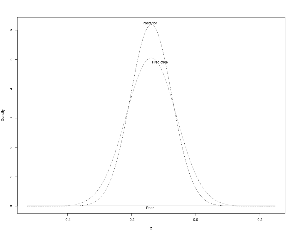
#Use unbiased prior with variance 1000 (almost flat)
b <- gbayes(0, 1000, m1, m2, stat, var.stat, 2*m1, 2*m2)
print(b)
plot(b)
#To get posterior Prob[parameter > w] use
# 1-pnorm(w, b$mean.post, sqrt(b$var.post))
#If g(effect, n1, n2) is the power function to
#detect an effect of 'effect' with samples size for groups 1 and 2
#of n1,n2, estimate the expected power by getting 1000 random
#draws from the posterior distribution, computing power for
#each value of the population effect, and averaging the 1000 powers
#This code assumes that g will accept vector-valued 'effect'
#For the 2-sample proportion problem just addressed, 'effect'
#could be taken approximately as the change in the arcsin of
#the square root of the probability of the event
g <- function(effect, n1, n2, alpha=.05) {
sd <- sqrt(var.stat(n1,n2))
z <- qnorm(1 - alpha/2)
effect <- abs(effect)
1 - pnorm(z - effect/sd) + pnorm(-z - effect/sd)
}
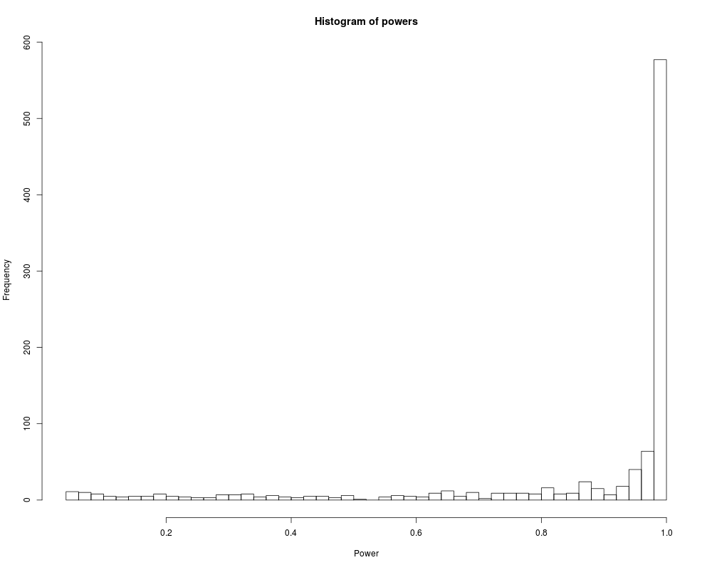
effects <- rnorm(1000, b$mean.post, sqrt(b$var.post))
powers <- g(effects, 500, 500)
hist(powers, nclass=35, xlab='Power')
describe(powers)
# gbayes2 examples
# First consider a study with a binary response where the
# sample size is n1=500 in the new treatment arm and n2=300
# in the control arm. The parameter of interest is the
# treated:control log odds ratio, which has variance
# 1/[n1 p1 (1-p1)] + 1/[n2 p2 (1-p2)]. This is not
# really constant so we average the variance over plausible
# values of the probabilities of response p1 and p2. We
# think that these are between .4 and .6 and we take a
# further short cut
v <- function(n1, n2, p1, p2) 1/(n1*p1*(1-p1)) + 1/(n2*p2*(1-p2))
n1 <- 500; n2 <- 300
ps <- seq(.4, .6, length=100)
vguess <- quantile(v(n1, n2, ps, ps), .75)
vguess
# 75%
# 0.02183459
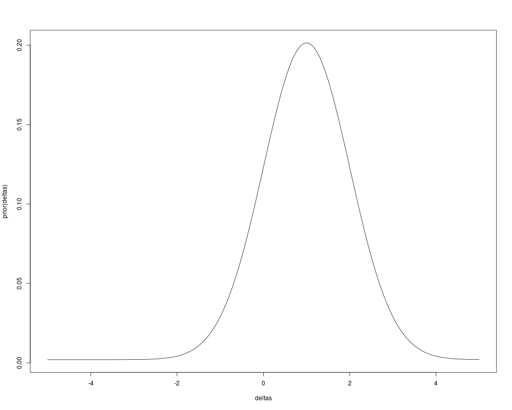
# The minimally interesting treatment effect is an odds ratio
# of 1.1. The prior distribution on the log odds ratio is
# a 50:50 mixture of a vague Gaussian (mean 0, sd 100) and
# an informative prior from a previous study (mean 1, sd 1)
prior <- function(delta)
0.5*dnorm(delta, 0, 100)+0.5*dnorm(delta, 1, 1)
deltas <- seq(-5, 5, length=150)
plot(deltas, prior(deltas), type='l')
# Now compute the power, averaged over this prior
gbayes2(sqrt(vguess), prior, log(1.1))
# [1] 0.6133338
# See how much power is lost by ignoring the previous
# study completely
gbayes2(sqrt(vguess), function(delta)dnorm(delta, 0, 100), log(1.1))
# [1] 0.4984588
# What happens to the power if we really don't believe the treatment
# is very effective? Let's use a prior distribution for the log
# odds ratio that is uniform between log(1.2) and log(1.3).
# Also check the power against a true null hypothesis
prior2 <- function(delta) dunif(delta, log(1.2), log(1.3))
gbayes2(sqrt(vguess), prior2, log(1.1))
# [1] 0.1385113
gbayes2(sqrt(vguess), prior2, 0)
# [1] 0.3264065
# Compare this with the power of a two-sample binomial test to
# detect an odds ratio of 1.25
bpower(.5, odds.ratio=1.25, n1=500, n2=300)
# Power
# 0.3307486
# For the original prior, consider a new study with equal
# sample sizes n in the two arms. Solve for n to get a
# power of 0.9. For the variance of the log odds ratio
# assume a common p in the center of a range of suspected
# probabilities of response, 0.3. For this example we
# use a zero null value and the uniform prior above
v <- function(n) 2/(n*.3*.7)
pow <- function(n) gbayes2(sqrt(v(n)), prior2)
uniroot(function(n) pow(n)-0.9, c(50,10000))$root
# [1] 2119.675
# Check this value
pow(2119.675)
# [1] 0.9
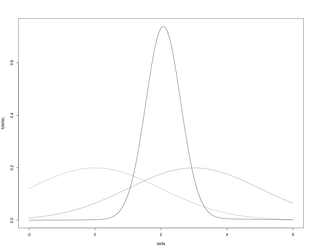
# Get the posterior density when there is a mixture of two priors,
# with mixing probability 0.5. The first prior is almost
# non-informative (normal with mean 0 and variance 10000) and the
# second has mean 2 and variance 0.3. The test statistic has a value
# of 3 with variance 0.4.
f <- gbayesMixPost(3, 4, mix=0.5, d0=0, v0=10000, d1=2, v1=0.3)
args(f)
# Plot this density
delta <- seq(-2, 6, length=150)
plot(delta, f(delta), type='l')
# Add to the plot the posterior density that used only
# the almost non-informative prior
lines(delta, f(delta, mix=1), lty=2)
# The same but for an observed statistic of zero
lines(delta, f(delta, mix=1, x=0), lty=3)
# Derive the CDF instead of the density
g <- gbayesMixPost(3, 4, mix=0.5, d0=0, v0=10000, d1=2, v1=0.3,
what='cdf')
# Had mix=0 or 1, gbayes1PowerNP could have been used instead
# of gbayesMixPowerNP below
# Compute the power to detect an effect of delta=1 if the variance
# of the test statistic is 0.2
gbayesMixPowerNP(g, 1, 0.2, interval=c(-10,12))
# Do the same thing by simulation
gbayesMixPowerNP(g, 1, 0.2, interval=c(-10,12), nsim=20000)
# Compute by what factor the sample size needs to be larger
# (the variance needs to be smaller) so that the power is 0.9
ratios <- seq(1, 4, length=50)
pow <- single(50)
for(i in 1:50)
pow[i] <- gbayesMixPowerNP(g, 1, 0.2/ratios[i], interval=c(-10,12))[2]
# Solve for ratio using reverse linear interpolation
approx(pow, ratios, xout=0.9)$y
# Check this by computing power
gbayesMixPowerNP(g, 1, 0.2/2.1, interval=c(-10,12))
# So the study will have to be 2.1 times as large as earlier thought
Results
R version 3.3.1 (2016-06-21) -- "Bug in Your Hair"
Copyright (C) 2016 The R Foundation for Statistical Computing
Platform: x86_64-pc-linux-gnu (64-bit)

R is free software and comes with ABSOLUTELY NO WARRANTY.
You are welcome to redistribute it under certain conditions.
Type 'license()' or 'licence()' for distribution details.

R is a collaborative project with many contributors.
Type 'contributors()' for more information and
'citation()' on how to cite R or R packages in publications.

Type 'demo()' for some demos, 'help()' for on-line help, or
'help.start()' for an HTML browser interface to help.
Type 'q()' to quit R.

> library(Hmisc)
Loading required package: lattice
Loading required package: survival
Loading required package: Formula
Loading required package: ggplot2

Attaching package: 'Hmisc'

The following objects are masked from 'package:base':

    format.pval, round.POSIXt, trunc.POSIXt, units

> png(filename="/home/ddbj/snapshot/RGM3/R_CC/result/Hmisc/gbayes.Rd_%03d_medium.png", width=480, height=480)
> ### Name: gbayes
> ### Title: Gaussian Bayesian Posterior and Predictive Distributions
> ### Aliases: gbayes plot.gbayes gbayes2 gbayesMixPredNoData gbayesMixPost
> ###   gbayesMixPowerNP gbayes1PowerNP
> ### Keywords: htest
>
> ### ** Examples
>
> # Compare 2 proportions using the var stabilizing transformation
> # arcsin(sqrt((x+3/8)/(n+3/4))) (Anscombe), which has variance
> # 1/[4(n+.5)]
>
>
> m1 <- 100;     m2 <- 150
> deaths1 <- 10; deaths2 <- 30
>
>
> f <- function(events,n) asin(sqrt((events+3/8)/(n+3/4)))
> stat <- f(deaths1,m1) - f(deaths2,m2)
> var.stat <- function(m1, m2) 1/4/(m1+.5) + 1/4/(m2+.5)
> cat("Test statistic:",format(stat),"  s.d.:",
+     format(sqrt(var.stat(m1,m2))), "\n")
Test statistic: -0.1388297   s.d.: 0.06441034
> #Use unbiased prior with variance 1000 (almost flat)
> b <- gbayes(0, 1000, m1, m2, stat, var.stat, 2*m1, 2*m2)
> print(b)
$mean.prior
[1] 0

$var.prior
[1] 1000

$mean.post
[1] -0.1388291

$var.post
[1] 0.004148675

$mean.pred
[1] -0.1388291

$var.pred
[1] 0.006227504

attr(,"class")
[1] "gbayes"
> plot(b)
> #To get posterior Prob[parameter > w] use
> # 1-pnorm(w, b$mean.post, sqrt(b$var.post))
>
>
> #If g(effect, n1, n2) is the power function to
> #detect an effect of 'effect' with samples size for groups 1 and 2
> #of n1,n2, estimate the expected power by getting 1000 random
> #draws from the posterior distribution, computing power for
> #each value of the population effect, and averaging the 1000 powers
> #This code assumes that g will accept vector-valued 'effect'
> #For the 2-sample proportion problem just addressed, 'effect'
> #could be taken approximately as the change in the arcsin of
> #the square root of the probability of the event
>
>
> g <- function(effect, n1, n2, alpha=.05) {
+   sd <- sqrt(var.stat(n1,n2))
+   z <- qnorm(1 - alpha/2)
+   effect <- abs(effect)
+   1 - pnorm(z - effect/sd) + pnorm(-z - effect/sd)
+ }
>
>
> effects <- rnorm(1000, b$mean.post, sqrt(b$var.post))
> powers <- g(effects, 500, 500)
> hist(powers, nclass=35, xlab='Power')
> describe(powers)
powers
      n missing  unique    Info    Mean     .05     .10     .25     .50     .75
   1000       0     998       1  0.8476  0.2053  0.4000  0.8170  0.9894  0.9999
    .90     .95
 1.0000  1.0000

lowest : 0.05005 0.05022 0.05132 0.05158 0.05219
highest: 1.00000 1.00000 1.00000 1.00000 1.00000
>
>
>
>
> # gbayes2 examples
> # First consider a study with a binary response where the
> # sample size is n1=500 in the new treatment arm and n2=300
> # in the control arm.  The parameter of interest is the
> # treated:control log odds ratio, which has variance
> # 1/[n1 p1 (1-p1)] + 1/[n2 p2 (1-p2)].  This is not
> # really constant so we average the variance over plausible
> # values of the probabilities of response p1 and p2.  We
> # think that these are between .4 and .6 and we take a
> # further short cut
>
>
> v <- function(n1, n2, p1, p2) 1/(n1*p1*(1-p1)) + 1/(n2*p2*(1-p2))
> n1 <- 500; n2 <- 300
> ps <- seq(.4, .6, length=100)
> vguess <- quantile(v(n1, n2, ps, ps), .75)
> vguess
       75%
0.02183459
> #        75%
> # 0.02183459
>
>
> # The minimally interesting treatment effect is an odds ratio
> # of 1.1.  The prior distribution on the log odds ratio is
> # a 50:50 mixture of a vague Gaussian (mean 0, sd 100) and
> # an informative prior from a previous study (mean 1, sd 1)
>
>
> prior <- function(delta)
+   0.5*dnorm(delta, 0, 100)+0.5*dnorm(delta, 1, 1)
> deltas <- seq(-5, 5, length=150)
> plot(deltas, prior(deltas), type='l')
>
>
> # Now compute the power, averaged over this prior
> gbayes2(sqrt(vguess), prior, log(1.1))
[1] 0.6133338
> # [1] 0.6133338
>
>
> # See how much power is lost by ignoring the previous
> # study completely
>
>
> gbayes2(sqrt(vguess), function(delta)dnorm(delta, 0, 100), log(1.1))
[1] 0.4984588
> # [1] 0.4984588
>
>
> # What happens to the power if we really don't believe the treatment
> # is very effective?  Let's use a prior distribution for the log
> # odds ratio that is uniform between log(1.2) and log(1.3).
> # Also check the power against a true null hypothesis
>
>
> prior2 <- function(delta) dunif(delta, log(1.2), log(1.3))
> gbayes2(sqrt(vguess), prior2, log(1.1))
[1] 0.1385113
> # [1] 0.1385113
>
>
> gbayes2(sqrt(vguess), prior2, 0)
[1] 0.3264065
> # [1] 0.3264065
>
>
> # Compare this with the power of a two-sample binomial test to
> # detect an odds ratio of 1.25
> bpower(.5, odds.ratio=1.25, n1=500, n2=300)
    Power
0.3307486
> #     Power
> # 0.3307486
>
>
> # For the original prior, consider a new study with equal
> # sample sizes n in the two arms.  Solve for n to get a
> # power of 0.9.  For the variance of the log odds ratio
> # assume a common p in the center of a range of suspected
> # probabilities of response, 0.3.  For this example we
> # use a zero null value and the uniform prior above
>
>
> v   <- function(n) 2/(n*.3*.7)
> pow <- function(n) gbayes2(sqrt(v(n)), prior2)
> uniroot(function(n) pow(n)-0.9, c(50,10000))$root
[1] 2119.688
> # [1] 2119.675
> # Check this value
> pow(2119.675)
[1] 0.8999984
> # [1] 0.9
>
>
> # Get the posterior density when there is a mixture of two priors,
> # with mixing probability 0.5.  The first prior is almost
> # non-informative (normal with mean 0 and variance 10000) and the
> # second has mean 2 and variance 0.3.  The test statistic has a value
> # of 3 with variance 0.4.
> f <- gbayesMixPost(3, 4, mix=0.5, d0=0, v0=10000, d1=2, v1=0.3)
>
>
> args(f)
function (delta = numeric(0), x = 3, v = 4, mix = 0.5, d0 = 0,
    v0 = 10000, d1 = 2, v1 = 0.3, dist = function (x, mean = 0,
        sd = 1, log = FALSE)
    .Call(C_dnorm, x, mean, sd, log))
NULL
>
>
> # Plot this density
> delta <- seq(-2, 6, length=150)
> plot(delta, f(delta), type='l')
>
>
> # Add to the plot the posterior density that used only
> # the almost non-informative prior
> lines(delta, f(delta, mix=1), lty=2)
>
>
> # The same but for an observed statistic of zero
> lines(delta, f(delta, mix=1, x=0), lty=3)
>
>
> # Derive the CDF instead of the density
> g <- gbayesMixPost(3, 4, mix=0.5, d0=0, v0=10000, d1=2, v1=0.3,
+                    what='cdf')
> # Had mix=0 or 1, gbayes1PowerNP could have been used instead
> # of gbayesMixPowerNP below
>
>
> # Compute the power to detect an effect of delta=1 if the variance
> # of the test statistic is 0.2
> gbayesMixPowerNP(g, 1, 0.2, interval=c(-10,12))
Critical value          Power
     0.5025818      0.8669870
>
>
> # Do the same thing by simulation
> gbayesMixPowerNP(g, 1, 0.2, interval=c(-10,12), nsim=20000)
     Power Lower 0.95 Upper 0.95
 0.8668000  0.8620907  0.8715093
>
>
> # Compute by what factor the sample size needs to be larger
> # (the variance needs to be smaller) so that the power is 0.9
> ratios <- seq(1, 4, length=50)
> pow <- single(50)
> for(i in 1:50)
+   pow[i] <- gbayesMixPowerNP(g, 1, 0.2/ratios[i], interval=c(-10,12))[2]
>
>
> # Solve for ratio using reverse linear interpolation
> approx(pow, ratios, xout=0.9)$y
[1] 1.214671
>
>
> # Check this by computing power
> gbayesMixPowerNP(g, 1, 0.2/2.1, interval=c(-10,12))
Critical value          Power
     0.4141731      0.9711715
> # So the study will have to be 2.1 times as large as earlier thought
>
>
>
>
>
> dev.off()
null device
          1
>
|