R Graphical Manual

Browse All

Last data update: 2014.03.03

R: Rank Correlation for Censored Data

rcorr.cens

R Documentation

Rank Correlation for Censored Data

Description

Computes the c index and the corresponding generalization of Somers' Dxy rank correlation for a censored response variable. Also works for uncensored and binary responses, although its use of all possible pairings makes it slow for this purpose. Dxy and c are related by var{Dxy} = 2*(var{c} - 0.5).

rcorr.cens handles one predictor variable. rcorrcens computes rank correlation measures separately by a series of predictors. In addition, rcorrcens has a rough way of handling categorical predictors. If a categorical (factor) predictor has two levels, it is coverted to a numeric having values 1 and 2. If it has more than 2 levels, an indicator variable is formed for the most frequently level vs. all others, and another indicator for the second most frequent level and all others. The correlation is taken as the maximum of the two (in absolute value).

Usage

rcorr.cens(x, S, outx=FALSE)

## S3 method for class 'formula'
rcorrcens(formula, data=NULL, subset=NULL,
          na.action=na.retain, exclude.imputed=TRUE, outx=FALSE,
          ...)

Arguments

`x`	a numeric predictor variable
`S`	an `Surv` object or a vector. If a vector, assumes that every observation is uncensored.
`outx`	set to `TRUE` to not count pairs of observations tied on `x` as a relevant pair. This results in a Goodman–Kruskal gamma type rank correlation.
`formula`	a formula with a `Surv` object or a numeric vector on the left-hand side
`data, subset, na.action`	the usual options for models. Default for `na.action` is to retain all values, NA or not, so that NAs can be deleted in only a pairwise fashion.
`exclude.imputed`	set to `FALSE` to include imputed values (created by `impute`) in the calculations.
`...`	extra arguments passed to `biVar`.

Value

rcorr.cens returns a vector with the following named elements: C Index, Dxy, S.D., n, missing, uncensored, Relevant Pairs, Concordant, and Uncertain

`n`	number of observations not missing on any input variables
`missing`	number of observations missing on `x` or `S`
`relevant`	number of pairs of non-missing observations for which `S` could be ordered
`concordant`	number of relevant pairs for which `x` and `S` are concordant.
`uncertain`	number of pairs of non-missing observations for which censoring prevents classification of concordance of `x` and `S`.

rcorrcens.formula returns an object of class biVar which is documented with the biVar function.

Author(s)

Frank Harrell
Department of Biostatistics
Vanderbilt University
f.harrell@vanderbilt.edu

References

Newson R: Confidence intervals for rank statistics: Somers' D and extensions. Stata Journal 6:309-334; 2006.

Examples

set.seed(1)
x <- round(rnorm(200))
y <- rnorm(200)
rcorr.cens(x, y, outx=TRUE)   # can correlate non-censored variables
library(survival)
age <- rnorm(400, 50, 10)
bp  <- rnorm(400,120, 15)
bp[1]  <- NA
d.time <- rexp(400)
cens   <- runif(400,.5,2)
death  <- d.time <= cens
d.time <- pmin(d.time, cens)
rcorr.cens(age, Surv(d.time, death))
r <- rcorrcens(Surv(d.time, death) ~ age + bp)
r
plot(r)

# Show typical 0.95 confidence limits for ROC areas for a sample size
# with 24 events and 62 non-events, for varying population ROC areas
# Repeat for 138 events and 102 non-events
set.seed(8)
par(mfrow=c(2,1))
for(i in 1:2) {
 n1 <- c(24,138)[i]
 n0 <- c(62,102)[i]
 y <- c(rep(0,n0), rep(1,n1))
 deltas <- seq(-3, 3, by=.25)
 C <- se <- deltas
 j <- 0
 for(d in deltas) {
  j <- j + 1
  x <- c(rnorm(n0, 0), rnorm(n1, d))
  w <- rcorr.cens(x, y)
  C[j]  <- w['C Index']
  se[j] <- w['S.D.']/2
 }
 low <- C-1.96*se; hi <- C+1.96*se
 print(cbind(C, low, hi))
 errbar(deltas, C, C+1.96*se, C-1.96*se,
        xlab='True Difference in Mean X',
        ylab='ROC Area and Approx. 0.95 CI')
 title(paste('n1=',n1,'  n0=',n0,sep=''))
 abline(h=.5, v=0, col='gray')
 true <- 1 - pnorm(0, deltas, sqrt(2))
 lines(deltas, true, col='blue')
}
par(mfrow=c(1,1))

Results


R version 3.3.1 (2016-06-21) -- "Bug in Your Hair"
Copyright (C) 2016 The R Foundation for Statistical Computing
Platform: x86_64-pc-linux-gnu (64-bit)

R is free software and comes with ABSOLUTELY NO WARRANTY.
You are welcome to redistribute it under certain conditions.
Type 'license()' or 'licence()' for distribution details.

R is a collaborative project with many contributors.
Type 'contributors()' for more information and
'citation()' on how to cite R or R packages in publications.

Type 'demo()' for some demos, 'help()' for on-line help, or
'help.start()' for an HTML browser interface to help.
Type 'q()' to quit R.

> library(Hmisc)
Loading required package: lattice
Loading required package: survival
Loading required package: Formula
Loading required package: ggplot2

Attaching package: 'Hmisc'

The following objects are masked from 'package:base':

    format.pval, round.POSIXt, trunc.POSIXt, units

> png(filename="/home/ddbj/snapshot/RGM3/R_CC/result/Hmisc/rcorr.cens.Rd_%03d_medium.png", width=480, height=480)
> ### Name: rcorr.cens
> ### Title: Rank Correlation for Censored Data
> ### Aliases: rcorr.cens rcorrcens rcorrcens.formula
> ### Keywords: survival nonparametric
> 
> ### ** Examples
> 
> set.seed(1)
> x <- round(rnorm(200))
> y <- rnorm(200)
> rcorr.cens(x, y, outx=TRUE)   # can correlate non-censored variables
       C Index            Dxy           S.D.              n        missing 
  4.762913e-01  -4.741744e-02   6.488578e-02   2.000000e+02   0.000000e+00 
    uncensored Relevant Pairs     Concordant      Uncertain 
  2.000000e+02   2.834400e+04   1.350000e+04   0.000000e+00 
> library(survival)
> age <- rnorm(400, 50, 10)
> bp  <- rnorm(400,120, 15)
> bp[1]  <- NA
> d.time <- rexp(400)
> cens   <- runif(400,.5,2)
> death  <- d.time <= cens
> d.time <- pmin(d.time, cens)
> rcorr.cens(age, Surv(d.time, death))
       C Index            Dxy           S.D.              n        missing 
  4.992573e-01  -1.485304e-03   3.673749e-02   4.000000e+02   0.000000e+00 
    uncensored Relevant Pairs     Concordant      Uncertain 
  2.790000e+02   1.333060e+05   6.655400e+04   2.629400e+04 
> r <- rcorrcens(Surv(d.time, death) ~ age + bp)
> r

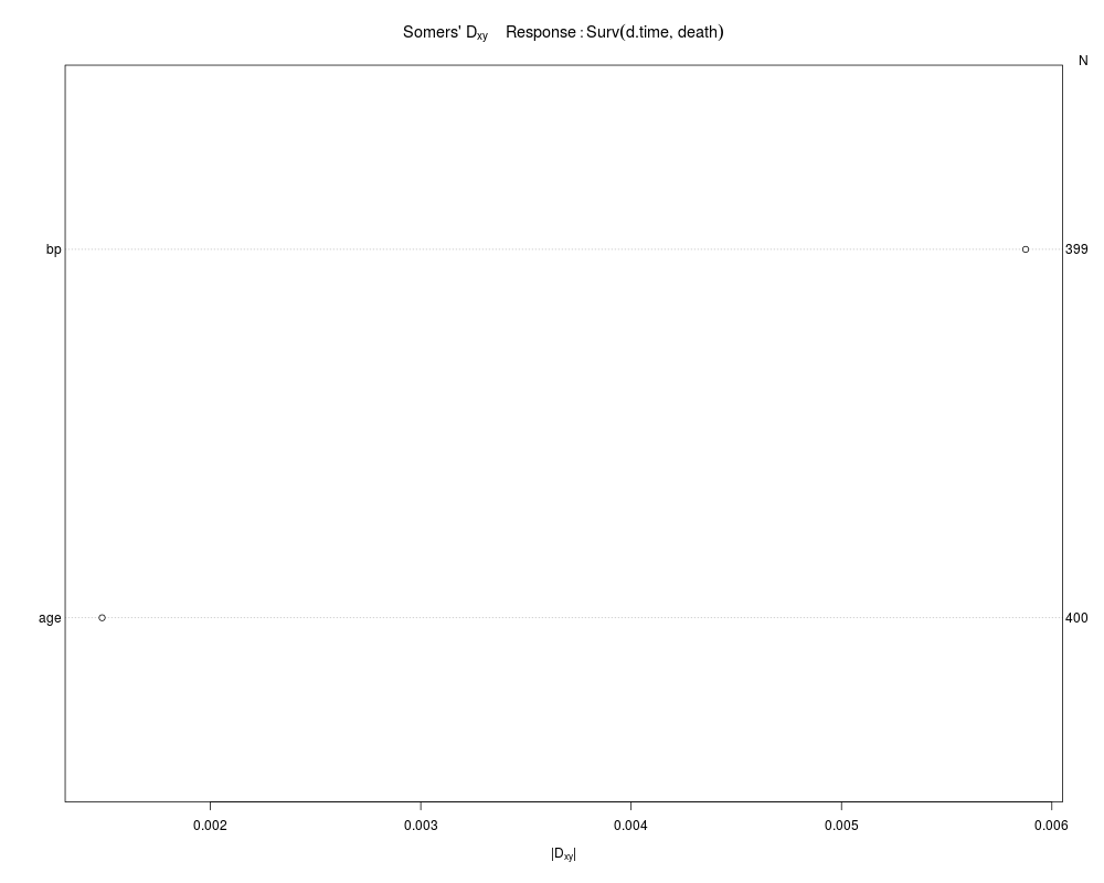
Somers' Rank Correlation for Censored Data    Response variable:Surv(d.time, death)

        C    Dxy  aDxy    SD    Z      P   n
age 0.499 -0.001 0.001 0.037 0.04 0.9678 400
bp  0.497 -0.006 0.006 0.038 0.15 0.8773 399
> plot(r)
> 
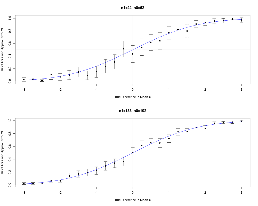
> # Show typical 0.95 confidence limits for ROC areas for a sample size
> # with 24 events and 62 non-events, for varying population ROC areas
> # Repeat for 138 events and 102 non-events
> set.seed(8)
> par(mfrow=c(2,1))
> for(i in 1:2) {
+  n1 <- c(24,138)[i]
+  n0 <- c(62,102)[i]
+  y <- c(rep(0,n0), rep(1,n1))
+  deltas <- seq(-3, 3, by=.25)
+  C <- se <- deltas
+  j <- 0
+  for(d in deltas) {
+   j <- j + 1
+   x <- c(rnorm(n0, 0), rnorm(n1, d))
+   w <- rcorr.cens(x, y)
+   C[j]  <- w['C Index']
+   se[j] <- w['S.D.']/2
+  }
+  low <- C-1.96*se; hi <- C+1.96*se
+  print(cbind(C, low, hi))
+  errbar(deltas, C, C+1.96*se, C-1.96*se,
+         xlab='True Difference in Mean X',
+         ylab='ROC Area and Approx. 0.95 CI')
+  title(paste('n1=',n1,'  n0=',n0,sep=''))
+  abline(h=.5, v=0, col='gray')
+  true <- 1 - pnorm(0, deltas, sqrt(2))
+  lines(deltas, true, col='blue')
+ }
               C           low         hi
 [1,] 0.02755376 -0.0015097885 0.05661732
 [2,] 0.03360215 -0.0003784209 0.06758272
 [3,] 0.01075269 -0.0044497156 0.02595509
 [4,] 0.10416667  0.0284823228 0.17985101
 [5,] 0.06787634  0.0142995376 0.12145315
 [6,] 0.09811828  0.0262850181 0.16995154
 [7,] 0.14717742  0.0687615968 0.22559324
 [8,] 0.09274194  0.0231499208 0.16233395
 [9,] 0.15322581  0.0606689017 0.24578271
[10,] 0.23857527  0.1324745070 0.34467603
[11,] 0.30846774  0.1940638328 0.42287165
[12,] 0.51411290  0.3856972238 0.64252858
[13,] 0.43346774  0.2978050069 0.56913048
[14,] 0.54099462  0.4094129537 0.67257629
[15,] 0.61357527  0.4861716011 0.74097894
[16,] 0.64180108  0.5083995705 0.77520258
[17,] 0.76948925  0.6660036397 0.87297485
[18,] 0.82325269  0.7183521941 0.92815318
[19,] 0.79771505  0.6891303373 0.90629977
[20,] 0.90793011  0.8496264055 0.96623381
[21,] 0.93615591  0.8826444375 0.98966739
[22,] 0.95766129  0.9218631555 0.99345943
[23,] 0.96303763  0.9280097068 0.99806556
[24,] 0.99059140  0.9780487323 1.00313406
[25,] 0.97177419  0.9353647894 1.00818360
               C         low         hi
 [1,] 0.02195226 0.006435429 0.03746909
 [2,] 0.02394146 0.009333689 0.03854923
 [3,] 0.02791986 0.011615456 0.04422427
 [4,] 0.06351236 0.033414116 0.09361061
 [5,] 0.06344132 0.034476786 0.09240585
 [6,] 0.13981245 0.094242001 0.18538289
 [7,] 0.17014777 0.119801626 0.22049391
 [8,] 0.19607843 0.140330050 0.25182681
 [9,] 0.22300369 0.164653945 0.28135344
[10,] 0.29560955 0.228818159 0.36240094
[11,] 0.33823529 0.268816721 0.40765387
[12,] 0.36608411 0.295661218 0.43650701
[13,] 0.50745951 0.433680623 0.58123839
[14,] 0.61530264 0.544122164 0.68648312
[15,] 0.65686275 0.588520795 0.72520469
[16,] 0.65231600 0.582394897 0.72223710
[17,] 0.72371412 0.659942480 0.78748577
[18,] 0.82551861 0.773470052 0.87756717
[19,] 0.82914180 0.778668043 0.87961556
[20,] 0.89386189 0.854440532 0.93328325
[21,] 0.88128730 0.840157819 0.92241678
[22,] 0.95865303 0.935219169 0.98208688
[23,] 0.97158284 0.954699265 0.98846641
[24,] 0.97428247 0.956007156 0.99255778
[25,] 0.98991191 0.981473900 0.99834991
> par(mfrow=c(1,1))
> 
> 
> 
> 
> 
> dev.off()
null device 
          1 
>