Supported by Dr. Osamu Ogasawara and  . . |
|
Last data update: 2014.03.03 |
Re-state Restricted Cubic Spline FunctionDescriptionThis function re-states a restricted cubic spline function in
the un-linearly-restricted form. Coefficients for that form are
returned, along with an R functional representation of this function
and a LaTeX character representation of the function.
Usage
rcspline.restate(knots, coef,
                 type=c("ordinary","integral"),
                 x="X", lx=nchar(x),
                 norm=2, columns=65, before="& &", after="\",
                 begin="", nbegin=0, digits=max(8, .Options$digits))

rcsplineFunction(knots, coef, norm=2, type=c('ordinary', 'integral'))
Arguments
Value
Author(s)Frank Harrell
See Also
Examples
set.seed(1)
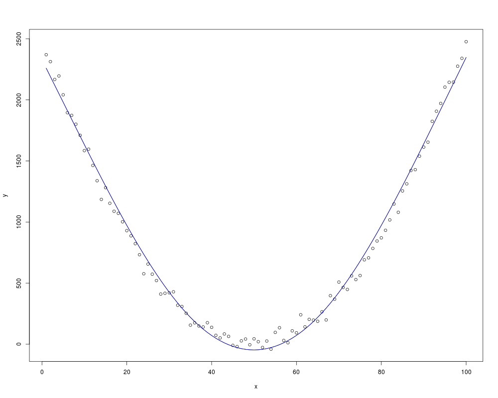
x <- 1:100
y <- (x - 50)^2 + rnorm(100, 0, 50)
plot(x, y)
xx <- rcspline.eval(x, inclx=TRUE, nk=4)
knots <- attr(xx, "knots")
coef <- lsfit(xx, y)$coef
options(digits=4)
# rcspline.restate must ignore intercept
w <- rcspline.restate(knots, coef[-1], x="{\rm BP}")
# could also have used coef instead of coef[-1], to include intercept
cat(attr(w,"latex"), sep="\n")
xtrans <- eval(attr(w, "function"))
# This is an S function of a single argument
lines(x, coef[1] + xtrans(x), type="l")
# Plots fitted transformation
xtrans <- rcsplineFunction(knots, coef)
xtrans
lines(x, xtrans(x), col='blue')
#x <- blood.pressure
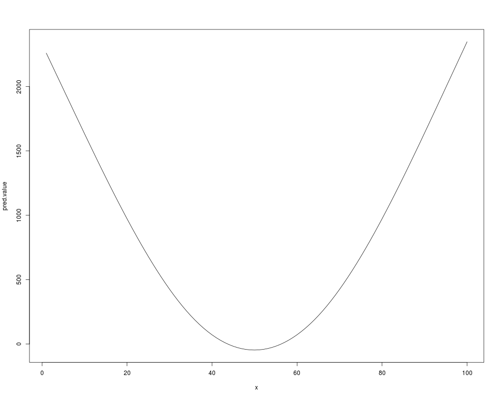
xx.simple <- cbind(x, pmax(x-knots[1],0)^3, pmax(x-knots[2],0)^3,
pmax(x-knots[3],0)^3, pmax(x-knots[4],0)^3)
pred.value <- coef[1] + xx.simple %*% w
plot(x, pred.value, type='l') # same as above
Results
R version 3.3.1 (2016-06-21) -- "Bug in Your Hair"
Copyright (C) 2016 The R Foundation for Statistical Computing
Platform: x86_64-pc-linux-gnu (64-bit)

R is free software and comes with ABSOLUTELY NO WARRANTY.
You are welcome to redistribute it under certain conditions.
Type 'license()' or 'licence()' for distribution details.

R is a collaborative project with many contributors.
Type 'contributors()' for more information and
'citation()' on how to cite R or R packages in publications.

Type 'demo()' for some demos, 'help()' for on-line help, or
'help.start()' for an HTML browser interface to help.
Type 'q()' to quit R.

> library(Hmisc)
Loading required package: lattice
Loading required package: survival
Loading required package: Formula
Loading required package: ggplot2

Attaching package: 'Hmisc'

The following objects are masked from 'package:base':

    format.pval, round.POSIXt, trunc.POSIXt, units

> png(filename="/home/ddbj/snapshot/RGM3/R_CC/result/Hmisc/rcspline.restate.Rd_%03d_medium.png", width=480, height=480)
> ### Name: rcspline.restate
> ### Title: Re-state Restricted Cubic Spline Function
> ### Aliases: rcspline.restate rcsplineFunction
> ### Keywords: regression interface character
>
> ### ** Examples
>
> set.seed(1)
> x <- 1:100
> y <- (x - 50)^2 + rnorm(100, 0, 50)
> plot(x, y)
> xx <- rcspline.eval(x, inclx=TRUE, nk=4)
> knots <- attr(xx, "knots")
> coef <- lsfit(xx, y)$coef
> options(digits=4)
> # rcspline.restate must ignore intercept
> w <- rcspline.restate(knots, coef[-1], x="{\rm BP}")
> # could also have used coef instead of coef[-1], to include intercept
> cat(attr(w,"latex"), sep="\n")
& & -69.685564  {
m BP}+0.013443742 ({
m BP}-5.95)_{+}^{3}
& & -0.013754656({
m BP}-35.65)_{+}^{3}-0.012821915({
m BP}-65.35)_{+}^{3}
& & +0.013132828 ({
m BP}-95.05)_{+}^{3}
>
>
> xtrans <- eval(attr(w, "function"))
> # This is an S function of a single argument
> lines(x, coef[1] + xtrans(x), type="l")
> # Plots fitted transformation
>
> xtrans <- rcsplineFunction(knots, coef)
> xtrans
function (x = numeric(0), knots = c(5.95, 35.65, 65.35, 95.05
), coef = c(2329.20175140574, -69.6855639459134, 106.727315060936,
-109.195599900753), kd = 19.9488777705554, type = "ordinary")
{
    k <- length(knots)
    knotnk <- knots[k]
    knotnk1 <- knots[k - 1]
    knot1 <- knots[1]
    if (length(coef) < k)
        coef <- c(0, coef)
    if (type == "ordinary") {
        y <- coef[1] + coef[2] * x
        for (j in 1:(k - 2)) y <- y + coef[j + 2] * (pmax((x -
            knots[j])/kd, 0)^3 + ((knotnk1 - knots[j]) * pmax((x -
            knotnk)/kd, 0)^3 - (knotnk - knots[j]) * (pmax((x -
            knotnk1)/kd, 0)^3))/(knotnk - knotnk1))
        return(y)
    }
    y <- coef[1] * x + 0.5 * coef[2] * x * x
    for (j in 1:(k - 2)) y <- y + 0.25 * coef[j + 2] * kd * (pmax((x -
        knots[j])/kd, 0)^4 + ((knotnk1 - knots[j]) * pmax((x -
        knotnk)/kd, 0)^4 - (knotnk - knots[j]) * (pmax((x - knotnk1)/kd,
        0)^4))/(knotnk - knotnk1))
    y
}
<environment: 0x43f3588>
> lines(x, xtrans(x), col='blue')
>
>
> #x <- blood.pressure
> xx.simple <- cbind(x, pmax(x-knots[1],0)^3, pmax(x-knots[2],0)^3,
+                        pmax(x-knots[3],0)^3, pmax(x-knots[4],0)^3)
> pred.value <- coef[1] + xx.simple %*% w
> plot(x, pred.value, type='l')   # same as above
>
>
>
>
>
> dev.off()
null device
          1
>
|