Supported by Dr. Osamu Ogasawara and  . . |
|
Last data update: 2014.03.03 |
Summarize Scalars or Matrices by Cross-ClassificationDescription
Usage
summarize(X, by, FUN, ...,
          stat.name=deparse(substitute(X)),
          type=c('variables','matrix'), subset=TRUE,
          keepcolnames=FALSE)

asNumericMatrix(x)

matrix2dataFrame(x, at=attr(x, 'origAttributes'), restoreAll=TRUE)
Arguments
ValueFor
Author(s)Frank Harrell
See Also
Examples
## Not run:
s <- summarize(ap>1, llist(size=cut2(sz, g=4), bone), mean,
stat.name='Proportion')
dotplot(Proportion ~ size | bone, data=s7)
## End(Not run)
set.seed(1)
temperature <- rnorm(300, 70, 10)
month <- sample(1:12, 300, TRUE)
year <- sample(2000:2001, 300, TRUE)
g <- function(x)c(Mean=mean(x,na.rm=TRUE),Median=median(x,na.rm=TRUE))
summarize(temperature, month, g)
mApply(temperature, month, g)
mApply(temperature, month, mean, na.rm=TRUE)
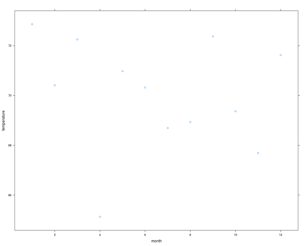
w <- summarize(temperature, month, mean, na.rm=TRUE)
library(lattice)
xyplot(temperature ~ month, data=w) # plot mean temperature by month
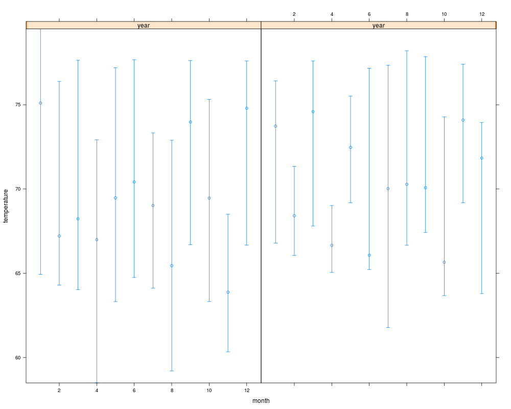
w <- summarize(temperature, llist(year,month),
quantile, probs=c(.5,.25,.75), na.rm=TRUE, type='matrix')
xYplot(Cbind(temperature[,1],temperature[,-1]) ~ month | year, data=w)
mApply(temperature, llist(year,month),
quantile, probs=c(.5,.25,.75), na.rm=TRUE)
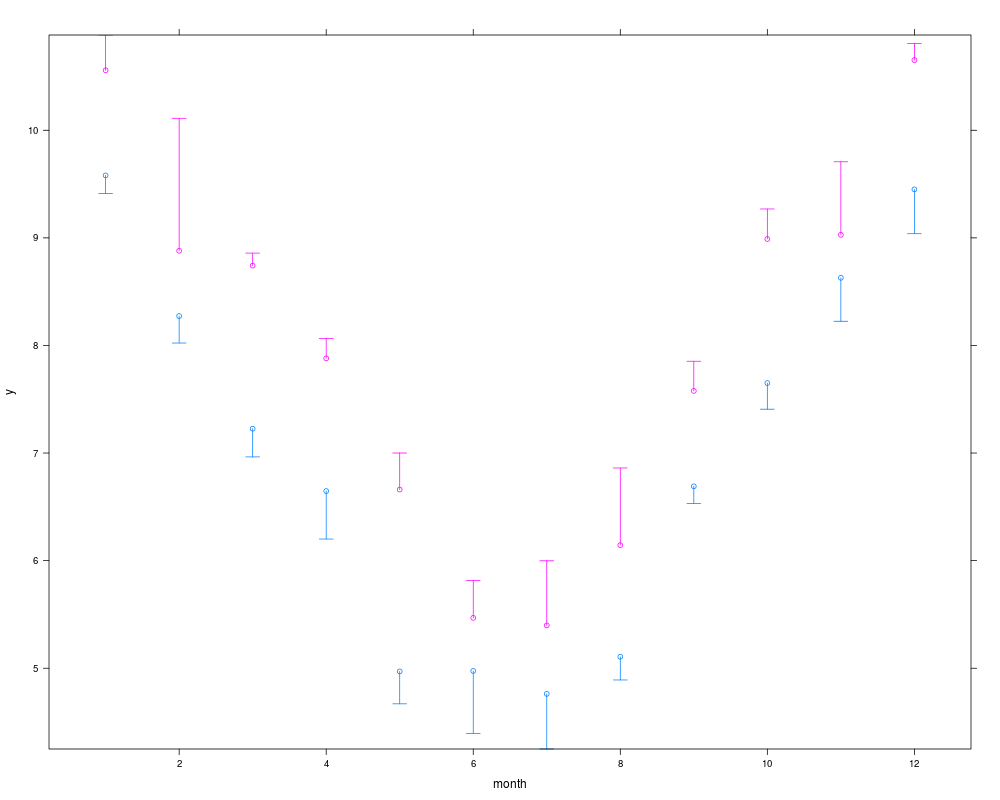
# Compute the median and outer quartiles. The outer quartiles are
# displayed using "error bars"
set.seed(111)
dfr <- expand.grid(month=1:12, year=c(1997,1998), reps=1:100)
attach(dfr)
y <- abs(month-6.5) + 2*runif(length(month)) + year-1997
s <- summarize(y, llist(month,year), smedian.hilow, conf.int=.5)
s
mApply(y, llist(month,year), smedian.hilow, conf.int=.5)
xYplot(Cbind(y,Lower,Upper) ~ month, groups=year, data=s,
keys='lines', method='alt')
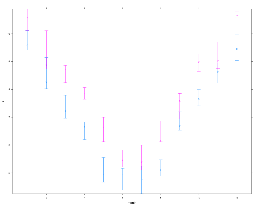
# Can also do:
s <- summarize(y, llist(month,year), quantile, probs=c(.5,.25,.75),
stat.name=c('y','Q1','Q3'))
xYplot(Cbind(y, Q1, Q3) ~ month, groups=year, data=s, keys='lines')
# To display means and bootstrapped nonparametric confidence intervals
# use for example:
s <- summarize(y, llist(month,year), smean.cl.boot)
xYplot(Cbind(y, Lower, Upper) ~ month | year, data=s)
# For each subject use the trapezoidal rule to compute the area under
# the (time,response) curve using the Hmisc trap.rule function
x <- cbind(time=c(1,2,4,7, 1,3,5,10),response=c(1,3,2,4, 1,3,2,4))
subject <- c(rep(1,4),rep(2,4))
trap.rule(x[1:4,1],x[1:4,2])
summarize(x, subject, function(y) trap.rule(y[,1],y[,2]))
## Not run:
# Another approach would be to properly re-shape the mm array below
# This assumes no missing cells. There are many other approaches.
# mApply will do this well while allowing for missing cells.
m <- tapply(y, list(year,month), quantile, probs=c(.25,.5,.75))
mm <- array(unlist(m), dim=c(3,2,12),
dimnames=list(c('lower','median','upper'),c('1997','1998'),
as.character(1:12)))
# aggregate will help but it only allows you to compute one quantile
# at a time; see also the Hmisc mApply function
dframe <- aggregate(y, list(Year=year,Month=month), quantile, probs=.5)
# Compute expected life length by race assuming an exponential
# distribution - can also use summarize
g <- function(y) { # computations for one race group
futime <- y[,1]; event <- y[,2]
sum(futime)/sum(event) # assume event=1 for death, 0=alive
}
mApply(cbind(followup.time, death), race, g)
# To run mApply on a data frame:
xn <- asNumericMatrix(x)
m <- mApply(xn, race, h)
# Here assume h is a function that returns a matrix similar to x
matrix2dataFrame(m)
# Get stratified weighted means
g <- function(y) wtd.mean(y[,1],y[,2])
summarize(cbind(y, wts), llist(sex,race), g, stat.name='y')
mApply(cbind(y,wts), llist(sex,race), g)
# Compare speed of mApply vs. by for computing
d <- data.frame(sex=sample(c('female','male'),100000,TRUE),
country=sample(letters,100000,TRUE),
y1=runif(100000), y2=runif(100000))
g <- function(x) {
y <- c(median(x[,'y1']-x[,'y2']),
med.sum =median(x[,'y1']+x[,'y2']))
names(y) <- c('med.diff','med.sum')
y
}
system.time(by(d, llist(sex=d$sex,country=d$country), g))
system.time({
x <- asNumericMatrix(d)
a <- subsAttr(d)
m <- mApply(x, llist(sex=d$sex,country=d$country), g)
})
system.time({
x <- asNumericMatrix(d)
summarize(x, llist(sex=d$sex, country=d$country), g)
})
# An example where each subject has one record per diagnosis but sex of
# subject is duplicated for all the rows a subject has. Get the cross-
# classified frequencies of diagnosis (dx) by sex and plot the results
# with a dot plot
count <- rep(1,length(dx))
d <- summarize(count, llist(dx,sex), sum)
Dotplot(dx ~ count | sex, data=d)
## End(Not run)
d <- list(x=1:10, a=factor(rep(c('a','b'),5)),
b=structure(letters[1:10], label='label for a'))
x <- asNumericMatrix(d)
attr(x, 'origAttributes')
matrix2dataFrame(x)
detach('dfr')
# Run summarize on a matrix to get column means
x <- c(1:19,NA)
y <- 101:120
z <- cbind(x, y)
g <- c(rep(1, 10), rep(2, 10))
summarize(z, g, colMeans, na.rm=TRUE, stat.name='x')
# Also works on an all numeric data frame
summarize(as.data.frame(z), g, colMeans, na.rm=TRUE, stat.name='x')
Results
R version 3.3.1 (2016-06-21) -- "Bug in Your Hair"
Copyright (C) 2016 The R Foundation for Statistical Computing
Platform: x86_64-pc-linux-gnu (64-bit)
R is free software and comes with ABSOLUTELY NO WARRANTY.
You are welcome to redistribute it under certain conditions.
Type 'license()' or 'licence()' for distribution details.
R is a collaborative project with many contributors.
Type 'contributors()' for more information and
'citation()' on how to cite R or R packages in publications.
Type 'demo()' for some demos, 'help()' for on-line help, or
'help.start()' for an HTML browser interface to help.
Type 'q()' to quit R.
> library(Hmisc)
Loading required package: lattice
Loading required package: survival
Loading required package: Formula
Loading required package: ggplot2
Attaching package: 'Hmisc'
The following objects are masked from 'package:base':
format.pval, round.POSIXt, trunc.POSIXt, units
> png(filename="/home/ddbj/snapshot/RGM3/R_CC/result/Hmisc/summarize.Rd_%03d_medium.png", width=480, height=480)
> ### Name: summarize
> ### Title: Summarize Scalars or Matrices by Cross-Classification
> ### Aliases: summarize asNumericMatrix matrix2dataFrame
> ### Keywords: category manip multivariate
>
> ### ** Examples
>
> ## Not run:
> ##D s <- summarize(ap>1, llist(size=cut2(sz, g=4), bone), mean,
> ##D stat.name='Proportion')
> ##D dotplot(Proportion ~ size | bone, data=s7)
> ## End(Not run)
>
> set.seed(1)
> temperature <- rnorm(300, 70, 10)
> month <- sample(1:12, 300, TRUE)
> year <- sample(2000:2001, 300, TRUE)
> g <- function(x)c(Mean=mean(x,na.rm=TRUE),Median=median(x,na.rm=TRUE))
> summarize(temperature, month, g)
month temperature Median
1 1 72.86559 73.76370
5 2 70.40988 68.01299
6 3 72.25304 72.23480
7 4 65.12354 66.99024
8 5 70.97783 70.69927
9 6 70.31975 67.41067
10 7 68.69374 69.32094
11 8 68.93415 69.43871
12 9 72.37940 72.07538
2 10 69.36739 68.64821
3 11 67.68554 68.60273
4 12 71.62634 73.29508
> mApply(temperature, month, g)
Mean Median
1 72.86559 73.76370
2 70.40988 68.01299
3 72.25304 72.23480
4 65.12354 66.99024
5 70.97783 70.69927
6 70.31975 67.41067
7 68.69374 69.32094
8 68.93415 69.43871
9 72.37940 72.07538
10 69.36739 68.64821
11 67.68554 68.60273
12 71.62634 73.29508
>
> mApply(temperature, month, mean, na.rm=TRUE)
1 2 3 4 5 6 7 8
72.86559 70.40988 72.25304 65.12354 70.97783 70.31975 68.69374 68.93415
9 10 11 12
72.37940 69.36739 67.68554 71.62634
> w <- summarize(temperature, month, mean, na.rm=TRUE)
> library(lattice)
> xyplot(temperature ~ month, data=w) # plot mean temperature by month
>
> w <- summarize(temperature, llist(year,month),
+ quantile, probs=c(.5,.25,.75), na.rm=TRUE, type='matrix')
> xYplot(Cbind(temperature[,1],temperature[,-1]) ~ month | year, data=w)
> mApply(temperature, llist(year,month),
+ quantile, probs=c(.5,.25,.75), na.rm=TRUE)
, , = 50%
year
month 2000 2001
1 75.10108 73.73195
2 67.20887 68.41245
3 68.22896 74.59516
4 66.99024 66.65822
5 69.47672 72.47187
6 70.42033 66.07192
7 69.01821 70.02132
8 65.44872 70.28002
9 73.98106 70.07726
10 69.46195 65.65376
11 63.87974 74.09402
12 74.79634 71.83643
, , = 25%
year
month 2000 2001
1 64.94043 66.78938
2 64.29278 66.05710
3 64.02734 67.80454
4 58.48734 65.04972
5 63.31722 69.19130
6 64.74534 65.21850
7 64.11106 61.77978
8 59.19621 66.65999
9 66.69092 67.41863
10 63.31821 63.67486
11 60.33722 69.18520
12 66.66562 63.79633
, , = 75%
year
month 2000 2001
1 79.51013 76.42336
2 76.39136 71.34448
3 77.64332 77.60490
4 72.92433 69.01739
5 77.20510 75.51480
6 77.67350 77.16707
7 73.32950 77.34330
8 72.90081 78.21221
9 77.63176 77.85528
10 75.31496 74.27858
11 68.50211 77.40600
12 77.60434 73.94379
>
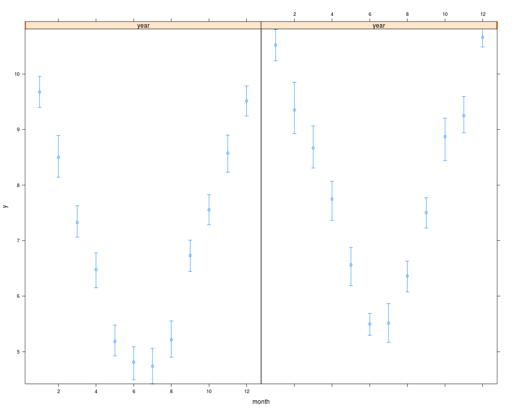
> # Compute the median and outer quartiles. The outer quartiles are
> # displayed using "error bars"
> set.seed(111)
> dfr <- expand.grid(month=1:12, year=c(1997,1998), reps=1:100)
> attach(dfr)
The following objects are masked _by_ .GlobalEnv:
month, year
> y <- abs(month-6.5) + 2*runif(length(month)) + year-1997
> s <- summarize(y, llist(month,year), smedian.hilow, conf.int=.5)
> s
month year y Lower Upper
7 1 2000 9.580386 9.410877 10.120838
8 1 2001 10.557353 10.112264 10.885294
9 2 2000 8.273255 8.022409 9.144197
10 2 2001 8.879700 8.732631 10.111084
11 3 2000 7.226451 6.964390 7.791556
12 3 2001 8.742167 8.244505 8.858170
13 4 2000 6.646968 6.200930 6.828694
14 4 2001 7.880373 7.644090 8.065150
15 5 2000 4.970555 4.669147 5.550791
16 5 2001 6.660632 6.120602 7.000524
17 6 2000 4.975022 4.393653 5.162116
18 6 2001 5.468378 5.219491 5.815384
19 7 2000 4.761814 4.249600 5.241279
20 7 2001 5.398562 5.109180 5.998700
21 8 2000 5.106799 4.891201 5.473976
22 8 2001 6.144053 6.117622 6.861511
23 9 2000 6.691147 6.529848 7.193447
24 9 2001 7.577245 6.934112 7.853399
1 10 2000 7.650484 7.407530 7.989939
2 10 2001 8.989472 8.646782 9.268328
3 11 2000 8.628861 8.224798 8.946738
4 11 2001 9.028428 8.748164 9.707166
5 12 2000 9.450670 9.038489 9.983661
6 12 2001 10.651994 10.566578 10.806413
> mApply(y, llist(month,year), smedian.hilow, conf.int=.5)
, , = Median
month
year 1 2 3 4 5 6 7 8
2000 9.580386 8.273255 7.226451 6.646968 4.970555 4.975022 4.761814 5.106799
2001 10.557353 8.879700 8.742167 7.880373 6.660632 5.468378 5.398562 6.144053
month
year 9 10 11 12
2000 6.691147 7.650484 8.628861 9.45067
2001 7.577245 8.989472 9.028428 10.65199
, , = Lower
month
year 1 2 3 4 5 6 7 8
2000 9.410877 8.022409 6.964390 6.20093 4.669147 4.393653 4.24960 4.891201
2001 10.112264 8.732631 8.244505 7.64409 6.120602 5.219491 5.10918 6.117622
month
year 9 10 11 12
2000 6.529848 7.407530 8.224798 9.038489
2001 6.934112 8.646782 8.748164 10.566578
, , = Upper
month
year 1 2 3 4 5 6 7 8
2000 10.12084 9.144197 7.791556 6.828694 5.550791 5.162116 5.241279 5.473976
2001 10.88529 10.111084 8.858170 8.065150 7.000524 5.815384 5.998700 6.861511
month
year 9 10 11 12
2000 7.193447 7.989939 8.946738 9.983661
2001 7.853399 9.268328 9.707166 10.806413
>
> xYplot(Cbind(y,Lower,Upper) ~ month, groups=year, data=s,
+ keys='lines', method='alt')
> # Can also do:
> s <- summarize(y, llist(month,year), quantile, probs=c(.5,.25,.75),
+ stat.name=c('y','Q1','Q3'))
> xYplot(Cbind(y, Q1, Q3) ~ month, groups=year, data=s, keys='lines')
> # To display means and bootstrapped nonparametric confidence intervals
> # use for example:
> s <- summarize(y, llist(month,year), smean.cl.boot)
> xYplot(Cbind(y, Lower, Upper) ~ month | year, data=s)
>
> # For each subject use the trapezoidal rule to compute the area under
> # the (time,response) curve using the Hmisc trap.rule function
> x <- cbind(time=c(1,2,4,7, 1,3,5,10),response=c(1,3,2,4, 1,3,2,4))
> subject <- c(rep(1,4),rep(2,4))
> trap.rule(x[1:4,1],x[1:4,2])
[1] 16
> summarize(x, subject, function(y) trap.rule(y[,1],y[,2]))
subject x
1 1 16
2 2 24
>
> ## Not run:
> ##D # Another approach would be to properly re-shape the mm array below
> ##D # This assumes no missing cells. There are many other approaches.
> ##D # mApply will do this well while allowing for missing cells.
> ##D m <- tapply(y, list(year,month), quantile, probs=c(.25,.5,.75))
> ##D mm <- array(unlist(m), dim=c(3,2,12),
> ##D dimnames=list(c('lower','median','upper'),c('1997','1998'),
> ##D as.character(1:12)))
> ##D # aggregate will help but it only allows you to compute one quantile
> ##D # at a time; see also the Hmisc mApply function
> ##D dframe <- aggregate(y, list(Year=year,Month=month), quantile, probs=.5)
> ##D
> ##D # Compute expected life length by race assuming an exponential
> ##D # distribution - can also use summarize
> ##D g <- function(y) { # computations for one race group
> ##D futime <- y[,1]; event <- y[,2]
> ##D sum(futime)/sum(event) # assume event=1 for death, 0=alive
> ##D }
> ##D mApply(cbind(followup.time, death), race, g)
> ##D
> ##D # To run mApply on a data frame:
> ##D xn <- asNumericMatrix(x)
> ##D m <- mApply(xn, race, h)
> ##D # Here assume h is a function that returns a matrix similar to x
> ##D matrix2dataFrame(m)
> ##D
> ##D
> ##D # Get stratified weighted means
> ##D g <- function(y) wtd.mean(y[,1],y[,2])
> ##D summarize(cbind(y, wts), llist(sex,race), g, stat.name='y')
> ##D mApply(cbind(y,wts), llist(sex,race), g)
> ##D
> ##D # Compare speed of mApply vs. by for computing
> ##D d <- data.frame(sex=sample(c('female','male'),100000,TRUE),
> ##D country=sample(letters,100000,TRUE),
> ##D y1=runif(100000), y2=runif(100000))
> ##D g <- function(x) {
> ##D y <- c(median(x[,'y1']-x[,'y2']),
> ##D med.sum =median(x[,'y1']+x[,'y2']))
> ##D names(y) <- c('med.diff','med.sum')
> ##D y
> ##D }
> ##D
> ##D system.time(by(d, llist(sex=d$sex,country=d$country), g))
> ##D system.time({
> ##D x <- asNumericMatrix(d)
> ##D a <- subsAttr(d)
> ##D m <- mApply(x, llist(sex=d$sex,country=d$country), g)
> ##D })
> ##D system.time({
> ##D x <- asNumericMatrix(d)
> ##D summarize(x, llist(sex=d$sex, country=d$country), g)
> ##D })
> ##D
> ##D # An example where each subject has one record per diagnosis but sex of
> ##D # subject is duplicated for all the rows a subject has. Get the cross-
> ##D # classified frequencies of diagnosis (dx) by sex and plot the results
> ##D # with a dot plot
> ##D
> ##D count <- rep(1,length(dx))
> ##D d <- summarize(count, llist(dx,sex), sum)
> ##D Dotplot(dx ~ count | sex, data=d)
> ## End(Not run)
> d <- list(x=1:10, a=factor(rep(c('a','b'),5)),
+ b=structure(letters[1:10], label='label for a'))
> x <- asNumericMatrix(d)
> attr(x, 'origAttributes')
$x
$x$ischar
[1] FALSE
$a
$a$levels
[1] "a" "b"
$a$class
[1] "factor"
$a$ischar
[1] FALSE
$b
$b$label
[1] "label for a"
$b$levels
[1] "a" "b" "c" "d" "e" "f" "g" "h" "i" "j"
$b$class
[1] "factor"
$b$ischar
[1] TRUE
> matrix2dataFrame(x)
x a b
1 1 a 1
2 2 b 2
3 3 a 3
4 4 b 4
5 5 a 5
6 6 b 6
7 7 a 7
8 8 b 8
9 9 a 9
10 10 b 10
>
> detach('dfr')
>
> # Run summarize on a matrix to get column means
> x <- c(1:19,NA)
> y <- 101:120
> z <- cbind(x, y)
> g <- c(rep(1, 10), rep(2, 10))
> summarize(z, g, colMeans, na.rm=TRUE, stat.name='x')
g x y
1 1 5.5 105.5
2 2 15.0 115.5
> # Also works on an all numeric data frame
> summarize(as.data.frame(z), g, colMeans, na.rm=TRUE, stat.name='x')
g x y
1 1 5.5 105.5
2 2 15.0 115.5
>
>
>
>
>
> dev.off()
null device
1
>
|