R Graphical Manual

Browse All

Last data update: 2014.03.03

R: IBD simulation

IBDsim

R Documentation

IBD simulation

Description

This is the main function of the package. Gene dropping of chromosomes is simulated down the pedigree, either unconditionally or conditional on the 'condition' pattern if this is given. Regions showing the 'query' pattern are collected and summarized.

Usage

IBDsim(x, sims, query=NULL, condition=NULL, map="decode", 
       chromosomes=NULL, model="chi", merged=TRUE, simdata=NULL, 
       skip.recomb = "noninf_founders", seed=NULL, verbose=TRUE)

Arguments

`x`	A pedigree in the form of a `linkdat` object.
`sims`	The number of simulations.
`query, condition`	Single allele patterns (SAPs), described as lists with numerical entries named "0", "1", "2", "atleast1", "atmost1".
`map`	The genetic map(s) to be used in the simulations: One of the character strings "decode", "uniform.sex.spec", "uniform.sex.aver". (See Details.)
`chromosomes`	A numeric vector indicating chromosome numbers, or either of the words "AUTOSOMAL" or "X". The default is 1:22, i.e. the human autosomes.
`model`	A character indicating the statistical model for recombination: Either "chi" (the default) or "haldane". (See details.)
`merged`	A logical, indicating if overlapping/adjacent regions should be merged or not.
`simdata`	Either NULL, in which case simulation is performed before collecting IBD regions, or an object containing simulation data (typically generated by a previous run of `IBDsim`).
`skip.recomb`	A numeric containing individuals whose meioses should be simulated without recombination (i.e. a random strand is passed on to each offspring). If NULL, nobody is skipped. The default value (the character "noninf_founders") computes the set of pedigree founders that cannot be carriers of the alleles described in the `condition` and/or `query` SAPs.
`seed`	NULL, or an integer to be passed on to `set.seed`).
`verbose`	A logical.

Details

Each simulation starts by unique alleles being distributed to the pedigree founders. In each subsequent meiosis, homologue chromosomes are made to recombine according to a renewal process along the four-strand bundle, with chi square distributed waiting times. (For comparison purposes, Haldane's Poisson model for recombination is also implemented.)

Recombination rates are sex-dependent, and vary along each chromosome according to the recombination map specified by the map parameter. By default, the complete Decode map of the human autosome is used (see References). If map="uniform.sex.spec", the genetic chromosome lengths are as in the Decode map, but the recombination rate is kept constant along each chromosome. If map="uniform.sex.aver", sex averaged genetic chromosome lengths are used (and constant recombination rates along each chromosome).

IBD patterns are described as combinations of Single Allele Patterns (SAPs). A SAP is a specification for a given allele of the number of copies carried by various individuals, and must be given as a list of numerical vectors (containing ID labels) named '0', '1', '2', 'atleast1' and 'atmost1' (some of these can be absent or NULL; see Examples).

If a condition SAP is given (i.e. if condition is non-null), simulation of each complete chromosome set (all autosomes by default) is performed as follows: A 'disease chromosome' is sampled at random (using the physical chromosome lengths as weights), followed by a random 'disease locus' on this chromosome. For this chromosome, gene dropping down the pedigree is carried out in such a way that the 'disease locus' has the condition SAP. (In a bit more detail: First, the program computes all possible sets of obligate carriers, with suitable weights, and samples one of these. Included in the obligate carriers will be exactly one founder, one of whose alleles is taken as the 'disease allele'. In each meiosis involving obligate carriers, recombination is performed as usual, but the strand carrying the 'disease allele' is always the one passed on.) For the other chromosomes, simulation is done unconditionally.

Value

If the query is NULL, no identification of IBD segments is done, and only the simulated genomes are (invisibly) returned.

If query is non-null, the segments with the query SAP are identified, and a list of three elements is returned. These are the 'simdata' (the simulated genomes), the 'segments' (a list of matrices describing all identified regions) and finally 'stats' (a matrix with one column per simulation, summarizing the regions from that genome). A summary is printed on the screen, with some or all of the following slots:

`count.all`	The average count of all IBD segments (i.e. counting both random regions and the disease region in case of conditional simulation).
`fraction.all`	The average fraction (in %) of the genome covered by IBD segments.
`average.all`	The average length (in Mb) of IBD segments.
`longest.all`	The average length (in Mb) of the longest IBD segment from each simulated genome.
`count.rand`	The average count of random IBD segments.
`fraction.rand`	The average fraction (in %) of the chromosomes covered by random IBD segments.
`average.rand`	The average length (in Mb) of random IBD segments.
`longest.rand`	The average length (in Mb) of the longest random IBD segment from each simulated genome.
`length.dis`	The average length of the disease segment (only with conditional simulation).
`rank.dis`	The average rank of the disease segment length among all the segments.
`zeroprob`	The percentage of simulations resulting in zero IBD segments.

The term 'IBD segment' in the above always refers to 'IBD segment matching the query SAP'. The suffixes .dis, .rand and .all points to respectively the disease IBD segments (only relevant in conditional simulations), the random, i.e. non-disease, IBD segments (only relevant in conditional simulations), and all IBD segments (in any simulation).

Author(s)

Magnus Dehli Vigeland

References

The Decode map:

Kong, A. et al. (2010) Fine scale recombination rate differences between sexes, populations and individuals. Nature, 467, 1099–1103. doi:10.1038/nature09525.

The chi-square model:

Zhao, H., Speed, T. P., McPeek, M. S. (1995) Statistical analysis of crossover interference using the chi-square model. Genetics, 139(2), 1045–1056.

Examples

# In all examples below, the 'sims' parameter is set to 1 to 
# decrease runtime. For realistic results increase to e.g. 1000.

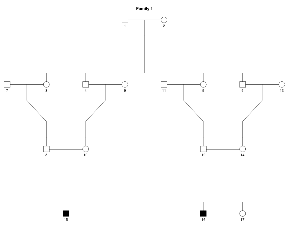
#### An example with a recessive disease in a consanguineous pedigree:

x = linkdat(twoloops)
plot(x)

# If individuals 15, 16 and 17 are available for sequencing, we can 
# predict the number and size of disease-compatible IBD segments as 
# follows:

sap1 = list('2'=15:16, 'atmost1'=17)
IBDsim(x, sims=1, condition=sap1, query=sap1)

# If 16 is unavailable, his parents and healthy sibling are still 
# informative. The regions we are looking for now are those with 
# an allele present in 2 copies in 15, 1 copy in 12 and 14, and 
# at most one in 17. Note that the condition SAP remains as above.

IBDsim(x, sims=1, condition=sap1, 
       query=list('2'=15, '1'=c(12,14), 'atmost1'=17))

	   
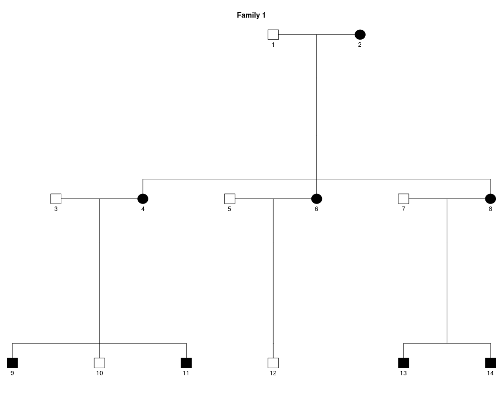
#### Example with an autosomal dominant disorder:
y = linkdat(dominant1) # lazy load data
plot(y)

# Suppose a 20 Mb linkage peak is found. 
# How often would this occur by chance?

aff = which(dominant1[,'AFF']==2)   # the affected
nonaff = which(dominant1[,'AFF']==1)   # the non-affected
dom_pattern = list('1'=aff, '0'=nonaff)
res = IBDsim(y, sims=1, query=dom_pattern) 
mean(res$stats['longest.all',] > 20)   # the estimated p-value


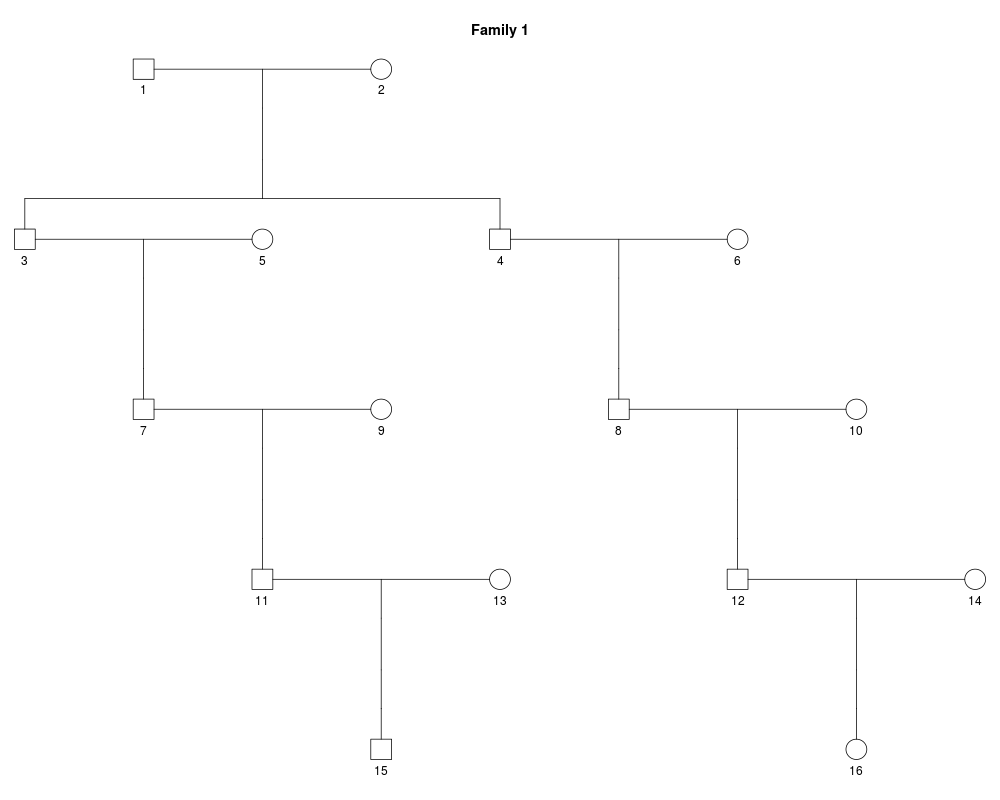
#### Another example: Unconditional simulation of regions shared 
# IBD by third cousins. The "zeroprob" entry in the output shows 
# the percentage of simulations having no IBD-sharing among the 
# two cousins. (Again: Increase 'sims' for more accurate results.)

x_male = cousinPed(3)
plot(x_male)
IBDsim(x_male, sims=1, query=list('1'=15:16))

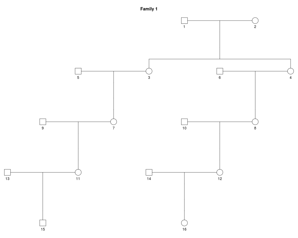
# Changing the genders of the individuals connecting the cousins 
# can have a big impact on the distribution of IBD segments:

x_female = swapSex(x_male, c(3,4,7,8,11,12))
plot(x_female)
IBDsim(x_female, sims=1, query=list('1'=15:16))

## Given that the two third cousins have at least one segment in 
# common, what is the expected length of this segment? We simulate 
# conditional on one allele in common between the cousins. The 
# "length.dis" entry of the summary shows the average length of 
# the disease region (which should be quite a lot larger than 
# an average random segment).

sap = list('1'=15:16)
IBDsim(x_male, sims=1, condition=sap, query=sap)


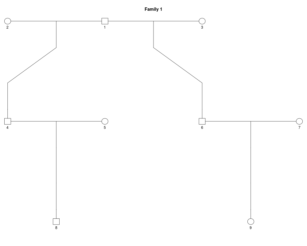
#### Let us look at a different relationship: Half first cousins. 
# Two such cousins will on average share 1/8 = 12.5% of the autosome.  

z = halfCousinPed(1)
plot(z)
res = IBDsim(z, sims=1, query=list('1'=8:9)) 
res$stats

# visualizing the spread in total IBD sharing and the number of segments:

IBD_percent = res$stats['fraction.all', ]
IBD_count = res$stats['count.all', ]
hist(IBD_percent) 
hist(IBD_count)

Results


R version 3.3.1 (2016-06-21) -- "Bug in Your Hair"
Copyright (C) 2016 The R Foundation for Statistical Computing
Platform: x86_64-pc-linux-gnu (64-bit)

R is free software and comes with ABSOLUTELY NO WARRANTY.
You are welcome to redistribute it under certain conditions.
Type 'license()' or 'licence()' for distribution details.

R is a collaborative project with many contributors.
Type 'contributors()' for more information and
'citation()' on how to cite R or R packages in publications.

Type 'demo()' for some demos, 'help()' for on-line help, or
'help.start()' for an HTML browser interface to help.
Type 'q()' to quit R.

> library(IBDsim)
Loading required package: paramlink
Loading required package: kinship2
Loading required package: Matrix
Loading required package: quadprog
> png(filename="/home/ddbj/snapshot/RGM3/R_CC/result/IBDsim/IBDsim.Rd_%03d_medium.png", width=480, height=480)
> ### Name: IBDsim
> ### Title: IBD simulation
> ### Aliases: IBDsim
> ### Keywords: math
> 
> ### ** Examples
> 
> # In all examples below, the 'sims' parameter is set to 1 to 
> # decrease runtime. For realistic results increase to e.g. 1000.
> 
> #### An example with a recessive disease in a consanguineous pedigree:
> 
> x = linkdat(twoloops)
Family ID: 1.
17 individuals.
2 affected 15 non-affected.
Loop(s) detected.
0 markers.

> plot(x)
> 
> # If individuals 15, 16 and 17 are available for sequencing, we can 
> # predict the number and size of disease-compatible IBD segments as 
> # follows:
> 
> sap1 = list('2'=15:16, 'atmost1'=17)
> IBDsim(x, sims=1, condition=sap1, query=sap1)
---------------
Performing conditional simulation
Mode: autosomal 
Recombination model: chi square renewal model 
Number of simulations: 1 
For the disease chromosome I'm sampling condition SAPs among the following:
SAP 1:
  Two copies: 15, 16 
  One copy: 1, 3, 4, 5, 6, 8, 10, 12, 14 
  At most one copy: 17 

SAP 2:
  Two copies: 15, 16 
  One copy: 2, 3, 4, 5, 6, 8, 10, 12, 14 
  At most one copy: 17 

Skipping recombination in the following individuals: 7, 9, 11, 13 
Simulation finished. Time used: 0.274 seconds
---------------

Inbreeding coefficients:
 ID      f
 15 0.0625
 16 0.0625
 17 0.0625

Results:
    count.all  fraction.all   average.all   longest.all    count.rand 
        2.000         0.965        13.823        25.805         1.000 
fraction.rand  average.rand  longest.rand    length.dis      rank.dis 
        0.064         1.840         1.840        25.805         1.000 
     zeroprob 
        0.000 

Total time used: 0.303 seconds.
> 
> # If 16 is unavailable, his parents and healthy sibling are still 
> # informative. The regions we are looking for now are those with 
> # an allele present in 2 copies in 15, 1 copy in 12 and 14, and 
> # at most one in 17. Note that the condition SAP remains as above.
> 
> IBDsim(x, sims=1, condition=sap1, 
+        query=list('2'=15, '1'=c(12,14), 'atmost1'=17))
---------------
Performing conditional simulation
Mode: autosomal 
Recombination model: chi square renewal model 
Number of simulations: 1 
For the disease chromosome I'm sampling condition SAPs among the following:
SAP 1:
  Two copies: 15, 16 
  One copy: 1, 3, 4, 5, 6, 8, 10, 12, 14 
  At most one copy: 17 

SAP 2:
  Two copies: 15, 16 
  One copy: 2, 3, 4, 5, 6, 8, 10, 12, 14 
  At most one copy: 17 

Skipping recombination in the following individuals: 7, 9, 11, 13 
Simulation finished. Time used: 0.122 seconds
---------------

Inbreeding coefficients:
 ID      f
 15 0.0625
 16 0.0625
 17 0.0625

Results:
    count.all  fraction.all   average.all   longest.all    count.rand 
        2.000         0.251         3.595         4.503         1.000 
fraction.rand  average.rand  longest.rand    length.dis      rank.dis 
        0.094         2.687         2.687         4.503         1.000 
     zeroprob 
        0.000 

Total time used: 0.148 seconds.
> 
> 	   
> #### Example with an autosomal dominant disorder:
> y = linkdat(dominant1) # lazy load data
Family ID: 1.
14 individuals.
8 affected 6 non-affected.
4 nuclear subfamilies.
0 markers.

> plot(y)
> 
> # Suppose a 20 Mb linkage peak is found. 
> # How often would this occur by chance?
> 
> aff = which(dominant1[,'AFF']==2)   # the affected
> nonaff = which(dominant1[,'AFF']==1)   # the non-affected
> dom_pattern = list('1'=aff, '0'=nonaff)
> res = IBDsim(y, sims=1, query=dom_pattern) 
---------------
Performing unconditional simulation
Mode: autosomal 
Recombination model: chi square renewal model 
Number of simulations: 1 
Skipping recombination in the following individuals: 1, 3, 5, 7 
Simulation finished. Time used: 0.064 seconds
---------------

Results:
   count.all fraction.all  average.all  longest.all     zeroprob 
           0            0            0            0          100 

Total time used: 0.127 seconds.
> mean(res$stats['longest.all',] > 20)   # the estimated p-value
[1] 0
> 
> 
> #### Another example: Unconditional simulation of regions shared 
> # IBD by third cousins. The "zeroprob" entry in the output shows 
> # the percentage of simulations having no IBD-sharing among the 
> # two cousins. (Again: Increase 'sims' for more accurate results.)
> 
> x_male = cousinPed(3)
> plot(x_male)
> IBDsim(x_male, sims=1, query=list('1'=15:16))
---------------
Performing unconditional simulation
Mode: autosomal 
Recombination model: chi square renewal model 
Number of simulations: 1 
Skipping recombination in the following individuals: 5, 6, 9, 10, 13, 14 
Simulation finished. Time used: 0.145 seconds
---------------

Results:
   count.all fraction.all  average.all  longest.all     zeroprob 
       2.000        1.027       14.715       20.898        0.000 

Total time used: 0.154 seconds.
> 
> # Changing the genders of the individuals connecting the cousins 
> # can have a big impact on the distribution of IBD segments:
> 
> x_female = swapSex(x_male, c(3,4,7,8,11,12))
Changing sex of the following spouses as well: 5, 6, 9, 10, 13, 14 
> plot(x_female)
> IBDsim(x_female, sims=1, query=list('1'=15:16))
---------------
Performing unconditional simulation
Mode: autosomal 
Recombination model: chi square renewal model 
Number of simulations: 1 
Skipping recombination in the following individuals: 5, 6, 9, 10, 13, 14 
Simulation finished. Time used: 0.061 seconds
---------------

Results:
   count.all fraction.all  average.all  longest.all     zeroprob 
       5.000        0.751        4.301       15.273        0.000 

Total time used: 0.076 seconds.
> 
> ## Given that the two third cousins have at least one segment in 
> # common, what is the expected length of this segment? We simulate 
> # conditional on one allele in common between the cousins. The 
> # "length.dis" entry of the summary shows the average length of 
> # the disease region (which should be quite a lot larger than 
> # an average random segment).
> 
> sap = list('1'=15:16)
> IBDsim(x_male, sims=1, condition=sap, query=sap)
---------------
Performing conditional simulation
Mode: autosomal 
Recombination model: chi square renewal model 
Number of simulations: 1 
For the disease chromosome I'm sampling condition SAPs among the following:
SAP 1:
  One copy: 1, 3, 4, 7, 8, 11, 12, 15, 16 

SAP 2:
  One copy: 2, 3, 4, 7, 8, 11, 12, 15, 16 

Skipping recombination in the following individuals: 5, 6, 9, 10, 13, 14 
Simulation finished. Time used: 0.059 seconds
---------------

Results:
    count.all  fraction.all   average.all   longest.all    count.rand 
        2.000         1.956        28.011        35.657         1.000 
fraction.rand  average.rand  longest.rand    length.dis      rank.dis 
        0.711        20.365        20.365        35.657         1.000 
     zeroprob 
        0.000 

Total time used: 0.067 seconds.
> 
> 
> #### Let us look at a different relationship: Half first cousins. 
> # Two such cousins will on average share 1/8 = 12.5% of the autosome.  
> 
> z = halfCousinPed(1)
> plot(z)
> res = IBDsim(z, sims=1, query=list('1'=8:9)) 
---------------
Performing unconditional simulation
Mode: autosomal 
Recombination model: chi square renewal model 
Number of simulations: 1 
Skipping recombination in the following individuals: 2, 3, 5, 7 
Simulation finished. Time used: 0.016 seconds
---------------

Results:
   count.all fraction.all  average.all  longest.all     zeroprob 
      12.000        7.516       17.940       63.398        0.000 

Total time used: 0.021 seconds.
> res$stats
                  [,1]
count.all    12.000000
fraction.all  7.515842
average.all  17.940307
longest.all  63.398452
> 
> # visualizing the spread in total IBD sharing and the number of segments:
> 
> IBD_percent = res$stats['fraction.all', ]
> IBD_count = res$stats['count.all', ]
> hist(IBD_percent) 
> hist(IBD_count)
> 
> 
> 
> 
> 
> dev.off()
null device 
          1 
>