Supported by Dr. Osamu Ogasawara and  . . |
|
Last data update: 2014.03.03 |
ConfigureIBHMDescriptionCreates a configuration object for Usage
ConfigureIBHM( stop.criterion = IterationSC(3),
         weighting.function = function(y, w.par){ 0.01+dnorm(y,sd=abs(w.par))},
         scal.optim = 'multi.CMAES',
         scal.optim.params = list(retries=3, inner=list(maxit=50, stopfitness=-1)),
         scal.candidates = c('dot.pr','radial','root.radial'),
         activ.optim = 'multi.CMAES',
         activ.optim.params = list(retries=3, inner=list(maxit=100, stopfitness=-1)),
         activ.candidates = c('tanh','logsig','lin'),
         jit=TRUE,
         verbose=FALSE,
         final.estimation = 'all',
         final.estimation.x = NULL,
         final.estimation.y = NULL,
         final.estimation.maxit = 100
       )
Arguments
DetailsThe model constructed by IBHM has the following form: f(x) = w_0 + ∑ w_i g(a_i h(x,d_i)+b_i) , where h:R^n->R is a scalarization function, g:R->R is an activation function, d_i is a parameter vector, and a_i, b_i, w_i are scalar parameters. The parameter estimation is based on optimizing weighted correlation measures between the model output and the approximation residual. This allows for an iterative model construction process which estimates both model structure and parameter values. For more details see [Zawistowski and Arabas]. ValueA configuration object for ReferencesZawistowski, P. and Arabas, J.: "Benchmarking IBHM method using NN3 competition dataset." In Proc. 6th int. conf. on Hybrid artificial intelligent systems - Vol. 1, HAIS'11, pp 263–270, 2011. Springer-Verlag. See Also
Examples
x <- seq(-3,3,length.out=400)
y <- tanh(x)
x.val <- runif(50,min=-6,max=6)
y.val <- tanh(x.val)
m <- TrainIBHM(x,y, ConfigureIBHM( scal.candidates = 'dot.pr',
activ.candidates = 'tanh',
stop.criterion = ValidationSC(x.val, y.val)))
summary(m)
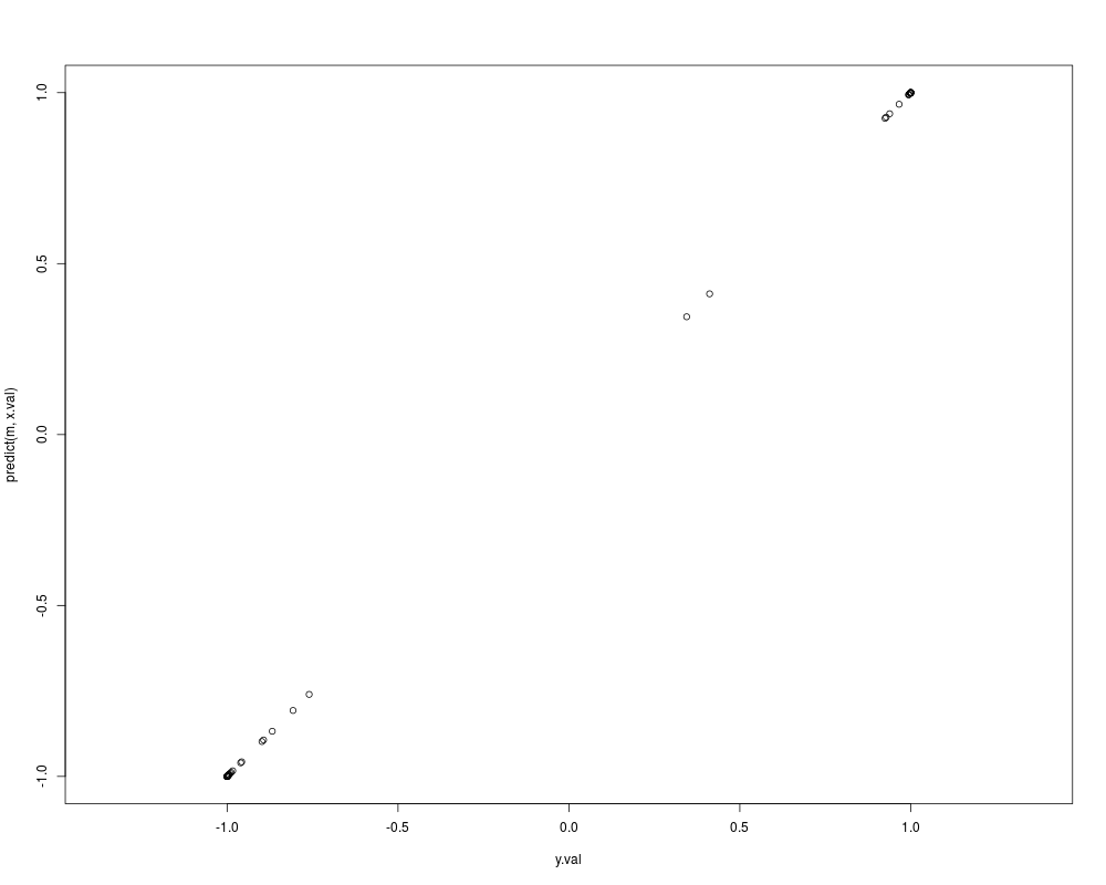
plot(y.val,predict(m,x.val),asp=1)
Results
R version 3.3.1 (2016-06-21) -- "Bug in Your Hair"
Copyright (C) 2016 The R Foundation for Statistical Computing
Platform: x86_64-pc-linux-gnu (64-bit)

R is free software and comes with ABSOLUTELY NO WARRANTY.
You are welcome to redistribute it under certain conditions.
Type 'license()' or 'licence()' for distribution details.

R is a collaborative project with many contributors.
Type 'contributors()' for more information and
'citation()' on how to cite R or R packages in publications.

Type 'demo()' for some demos, 'help()' for on-line help, or
'help.start()' for an HTML browser interface to help.
Type 'q()' to quit R.

> library(IBHM)
Loading required package: compiler
Loading required package: DEoptim

DEoptim package
Differential Evolution algorithm in R
Authors: D. Ardia, K. Mullen, B. Peterson and J. Ulrich

Loading required package: cmaes
Loading required package: Rcpp
> png(filename="/home/ddbj/snapshot/RGM3/R_CC/result/IBHM/ConfigureIBHM.Rd_%03d_medium.png", width=480, height=480)
> ### Name: ConfigureIBHM
> ### Title: ConfigureIBHM
> ### Aliases: ConfigureIBHM
> ### Keywords: ~models ~regression ~nonlinear
>
> ### ** Examples
>
>   x <- seq(-3,3,length.out=400)
>   y <- tanh(x)
>
>   x.val <- runif(50,min=-6,max=6)
>   y.val <- tanh(x.val)
>
>   m <- TrainIBHM(x,y, ConfigureIBHM(  scal.candidates = 'dot.pr',
+                                       activ.candidates = 'tanh',
+                                       stop.criterion = ValidationSC(x.val, y.val)))
Note: no visible binding for global variable '.refClassDef'
Note: no visible binding for global variable '.refClassDef'
Note: no visible binding for global variable '.pointer'
Note: no visible binding for global variable '.pointer'
Note: no visible binding for global variable '.pointer'
>
>   summary(m)
Model equation:  -1.43e-03 + 1.00e+00 tanh  ( 1.40e+00 * dot.pr (x,[ -2.16e+00 7.12e-01 ]) + 3.03e+00 )   -1.50e-03 tanh  ( 3.00e+00 * dot.pr (x,[ 5.34e-02 -4.56e-02 ]) + -2.12e+00 )
 Model size:  2

 Train set dim:  1  Train set size:  400
 MSE:   2.536345e-11  Std. dev:
 RMSE:  5.036214e-06
 Pearson correlation coefficient:  1
>   plot(y.val,predict(m,x.val),asp=1)
>
>
>
>
>
>
> dev.off()
null device
          1
>
Note: no visible binding for global variable '.pointer'
|