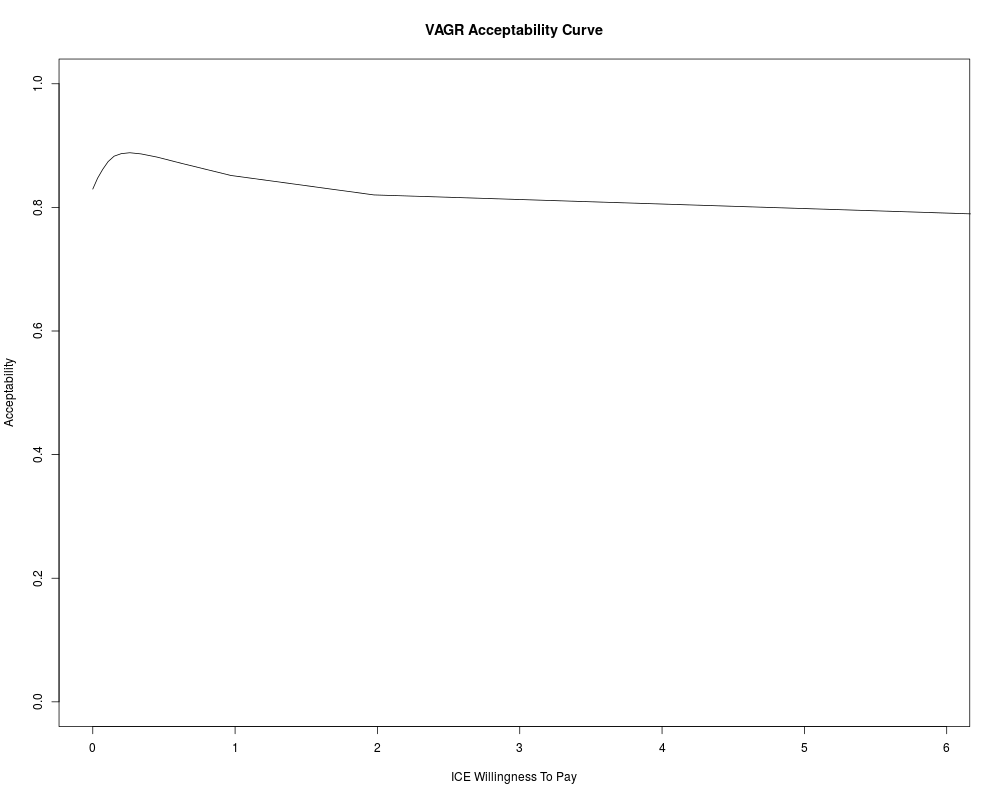
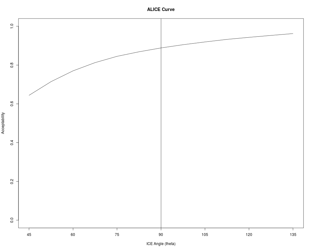
Functions to compute and display ICE Acceptability Curves

Description

ICEalice() computes statistics for the VAGR Acceptability Curve and for the Buckingham ALICE curve. Plots for the resulting ICEalice object are of two types: [1] a VAGR curve where the horizontal axis is the Willingness to Pay (WTP) ICE Ratio, and [2] a monotone ALICE curve where the horizontal axis is the Absolute Value of the ICE Polar Angle, which varies from +45 degrees to +135 degrees. Printing an ICEalice object yields a 13 x 5 table (matrix) of numerical values for Absolute ICEangle, WTP, VAGR Acceptability, WTA and ALICE acceptability, respectively.

Usage

 ICEalice(ICEw)

Arguments

Details

The VAGR Acceptability Curve displays the fraction of outcomes within the Bootstrap distribution of ICE Uncertainty that lie below and/or to the right of a rotating straight line through the origin of the ICE plane. This straight line starts out horizontal, representing lambda = WTP = 0, and rotates counter-clockwise until it becomes vertical, representing lambda = WTP = +Inf.

The Buckingham ALICE Curve assumes that lambra is held fixed. It displays the fraction of outcomes within the Bootstrap distribution of ICE Uncertainty that lie on or between a pair of rotating ICE rays (eminating from the ICE origin) with slopes representing KINKed values of WTP < WTA that always satisfy Obenchain's LINK function, lambda = sqrt(WTP*WTA), with lambda held fixed. The right-hand ray for WTP starts out horizontal and pointing to the right, then rotates counter-clockwise until it is vertical, as in a VAGR curve. The left-hand ray for WTA starts out vertical and pointing downwards, then rotates clockwise until it is horizontal. Since lambda is held fixed, the slopes of the rotating rays corresponding to decreasing WTA as WTP increases. The starting point of an ALICE curve at an Absolute ICE Angle of 45 degrees always represents the fraction of outcomes in the Bootstrap Distribution of ICE Uncertainty for which the new treatment is both less costly AND more effective than the std treatment. The ending point of an ALICE curve at an Absolute ICE Angle of 135 degrees always represents the fraction of outcomes in the Bootstrap Distribution of ICE Uncertainty for which the new treatment is either less costly OR more effective than the std treatment. The middle point of an ALICE curve at an Absolute ICE Angle of 90 degrees represents the fraction of outcomes in the Bootstrap Distribution of ICE Uncertainty falling below and/or to the right of the straight line through the ICE origin of slope lambda = WTP = WTA.

Value

Objects of class ICEalice contain the following output list:

Author(s)

Bob Obenchain <wizbob@att.net>

References

Van Hout BA, Al MJ, Gordon GS, Rutten FFH. Costs, effects and C/E ratios alongside a clinical trial. (VAGR curve) Health Economics 1994; 3: 309-319.

Buckingham K. Personal communications including a draft manuscript entitled: Representing the cumulative probability of Acceptability Levels In Cost Effectiveness. (ALICE curve) 2003.

Fenwick E, O'Brien BJ, Briggs AH. Cost-effectiveness acceptability curves - facts, fallacies and frequently asked questions. Health Economics 2004; 13: 405-415.

Obenchain RL. ICE Preference Maps: Nonlinear Generalizations of Net Benefit and Acceptability. Health Serv Outcomes Res Method 2008; 8: 31-56. DOI 10.1007/s10742-007-0027-2. Open Access.

Obenchain RL. ICEinR.pdf Vignette-like documentation for ICEinfer stored in the R library/ICEinfer/doc folder. 2009; 30 pages.

See Also

ICEwedge and ICEcolor

Examples

  # Read in previously computed ICEwedge output list.
  data(dpwdg)
  dpacc <- ICEalice(dpwdg)
  # Display VAGR and ALICE acceptability curves.
  plot(dpacc)

Results

R version 3.3.1 (2016-06-21) -- "Bug in Your Hair"
Copyright (C) 2016 The R Foundation for Statistical Computing
Platform: x86_64-pc-linux-gnu (64-bit)

R is free software and comes with ABSOLUTELY NO WARRANTY.
You are welcome to redistribute it under certain conditions.
Type 'license()' or 'licence()' for distribution details.

R is a collaborative project with many contributors.
Type 'contributors()' for more information and
'citation()' on how to cite R or R packages in publications.

Type 'demo()' for some demos, 'help()' for on-line help, or
'help.start()' for an HTML browser interface to help.
Type 'q()' to quit R.

> library(ICEinfer)
Loading required package: lattice
> png(filename="/home/ddbj/snapshot/RGM3/R_CC/result/ICEinfer/ICEalice.Rd_%03d_medium.png", width=480, height=480)
> ### Name: ICEalice
> ### Title: Functions to compute and display ICE Acceptability Curves
> ### Aliases: ICEalice
> ### Keywords: methods
> 
> ### ** Examples
> 
>   # Read in previously computed ICEwedge output list.
>   data(dpwdg)
>   dpacc <- ICEalice(dpwdg)
>   # Display VAGR and ALICE acceptability curves.
>   plot(dpacc)
> 
> 
> 
> 
> 
> dev.off()
null device 
          1 
>