ICE Statistical Inference and Economic Preference Variation

Description

Functions in the ICE Statistical Inference package make head-to-head comparisons between patients in two treatment cohorts (assumed to be unbiased samples) in two distinct dimensions, cost and effectiveness.

Bootstrap resampling methods quantify the endogenous Distribution of ICE Uncertainty and define Wedge-Shaped Statistical Confidence Regions equivariant relative to exogenous choice for the numerical Shadow Price of Health, lambda.

Preference maps with (linear or nonlinear) indiference curves can be viewed or superimposed upon endogenous confidence wedges to illustrate that considerable additional, potentially self-contradictory Economic Preference Uncertainty results from deliberately varying lambda.

Details

Statistical inference using functions from the ICEinfer package usually start with (possibly multiple) invocations of ICEscale() to help determine a reasonable value for the Shadow Price of Health, lambda. This is invariably followed by a single call to ICEuncrt to generate the Bootstrap Distribution of ICE Uncertainty corresponding to the chosen value of lambda. However, the print() and plot() functions for objects of type ICEuncrt do have optional arguments, lfact and swu, to help the user quantify and visualize the consequences of changing lambda and switching between cost and effe units.

Next, a single call to ICEwedge() yields the equivariant, wedge-shaped region of specified statistical confidence within [.50, .99] ...by computing ICE Angle Order Statistics around a circle centered at the ICE Origin, (DeltaEffe, DeltaCost) = (0, 0).

Researchers wishing to view alternative ICE Acceptability Curves would then envoke ICEalice().

Finally, multiple calls to ICEcolor for different values of lambda and/or different forms of (linear or nonlinear) ICE Preference Maps are typically used to illustrate the considerable additional Economic Preference Uncertainty that can be introduced. This Economic Uncertainty is superimposed on top of the inherent Statistical Uncertainty contained in unbiased, patient level data on the relative cost and effectiveness of two treatments for the same disease / condition.

Author(s)

Bob Obenchain <wizbob@att.net>

References

Black WC. The CE plane: a graphic representation of cost-effectiveness. Med Decis Making 1990; 10: 212-214.

Laupacis A, Feeny D, Detsky AS, Tugwell PX. How attractive does a new technology have to be to warrant adoption and utilization? Tentative guidelines for using clinical and economic evaluations. Can Med Assoc J 1992; 146(4): 473-81.

Stinnett AA, Mullahy J. Net health benefits: a new framework for the analysis of uncertainty in cost-effectiveness analysis. Medical Decision Making, Special Issue on Pharmacoeconomics 1998; 18: S68-S80.

O'Brien B, Gersten K, Willan A, Faulkner L. Is there a kink in consumers' threshold value for cost-effectiveness in health care? Health Econ 2002; 11: 175-180.

Obenchain RL. ICE Preference Maps: Nonlinear Generalizations of Net Benefit and Acceptability. Health Serv Outcomes Res Method 2008; 8: 31-56. DOI 10.1007/s10742-007-0027-2. Open Access.

Obenchain RL. ICEinR.pdf Vignette-like documentation for ICEinfer stored in the R library/ICEinfer/doc folder. 2009; 30 pages.

Examples

  demo(dulxparx)

Results

R version 3.3.1 (2016-06-21) -- "Bug in Your Hair"
Copyright (C) 2016 The R Foundation for Statistical Computing
Platform: x86_64-pc-linux-gnu (64-bit)

R is free software and comes with ABSOLUTELY NO WARRANTY.
You are welcome to redistribute it under certain conditions.
Type 'license()' or 'licence()' for distribution details.

R is a collaborative project with many contributors.
Type 'contributors()' for more information and
'citation()' on how to cite R or R packages in publications.

Type 'demo()' for some demos, 'help()' for on-line help, or
'help.start()' for an HTML browser interface to help.
Type 'q()' to quit R.

> library(ICEinfer)
Loading required package: lattice
> png(filename="/home/ddbj/snapshot/RGM3/R_CC/result/ICEinfer/ICEinfer-package.Rd_%03d_medium.png", width=480, height=480)
> ### Name: ICEinfer-package
> ### Title: ICE Statistical Inference and Economic Preference Variation
> ### Aliases: ICEinfer-package
> ### Keywords: package
> 
> ### ** Examples
> 
>   demo(dulxparx)


	demo(dulxparx)
	---- ~~~~~~~~

> require(ICEinfer)

> # input the dulxparx data of Obenchain et al. (2000).
> data(dulxparx)

> # Effectiveness = idb, Cost = ru, trtm = dulx where
> # dulx = 1 ==> Duloxetine treatment and dulx = 0 ==> Paroxetine treatment
> #
> # Display of Lambda => Shadow Price Summary Statistics...
> ICEscale(dulxparx, dulx, idb, ru)

Incremental Cost-Effectiveness (ICE) Lambda Scaling Statistics

Specified Value of Lambda   = 1
Cost and Effe Differences are both expressed in cost units

Effectiveness variable Name = idb
     Cost     variable Name = ru
  Treatment   factor   Name = dulx
New treatment level is = 1 and Standard level is = 0 

Observed  Treatment Diff = 6.152
Std. Error of Trtm Diff  = 8.186 

Observed Cost Difference = -2.899
Std. Error of Cost Diff  = 3.096 

Observed  ICE  Ratio     = -0.471 

Statistical Shadow Price = 0.378
Power-of-Ten Shadow Price= 1 


> ICEscale(dulxparx, dulx, idb, ru, lambda=0.26)

Incremental Cost-Effectiveness (ICE) Lambda Scaling Statistics

Specified Value of Lambda   = 0.26
Cost and Effe Differences are both expressed in cost units

Effectiveness variable Name = idb
     Cost     variable Name = ru
  Treatment   factor   Name = dulx
New treatment level is = 1 and Standard level is = 0 

Observed  Treatment Diff = 1.6
Std. Error of Trtm Diff  = 2.128 

Observed Cost Difference = -2.899
Std. Error of Cost Diff  = 3.096 

Observed  ICE  Ratio     = -1.812 

Statistical Shadow Price = 1.455
Power-of-Ten Shadow Price= 1 


> # Bootstrap ICE Uncertainty calculations can be time consuming...
> dpunc <- ICEuncrt(dulxparx, dulx, idb, ru, R = 10000, lambda=0.26)

> dpunc

Incremental Cost-Effectiveness (ICE) Bivariate Bootstrap Uncertainty

Shadow Price = Lambda = 0.26
Bootstrap Replications, R = 10000
Effectiveness variable Name = idb
     Cost     variable Name = ru
  Treatment   factor   Name = dulx
New treatment level is = 1 and Standard level is = 0 

Cost and Effe Differences are both expressed in cost units

Observed  Treatment Diff = 1.6
Mean Bootstrap Trtm Diff = 1.593 

Observed Cost Difference = -2.899
Mean Bootstrap Cost Diff = -2.88 


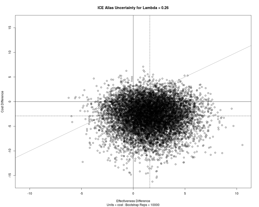
> # Display the Bootstrap ICE Uncertainty Distribution...
> plot(dpunc)

Incremental Cost-Effectiveness (ICE) Bivariate Bootstrap Uncertainty

Shadow Price = Lambda = 0.26
Bootstrap Replications, R = 10000
Effectiveness variable Name = idb
     Cost     variable Name = ru
  Treatment   factor   Name = dulx
New treatment level is = 1 and Standard level is = 0 

Cost and Effe Differences are both expressed in cost units

Observed  Treatment Diff = 1.6
Mean Bootstrap Trtm Diff = 1.593 

Observed Cost Difference = -2.899
Mean Bootstrap Cost Diff = -2.88 


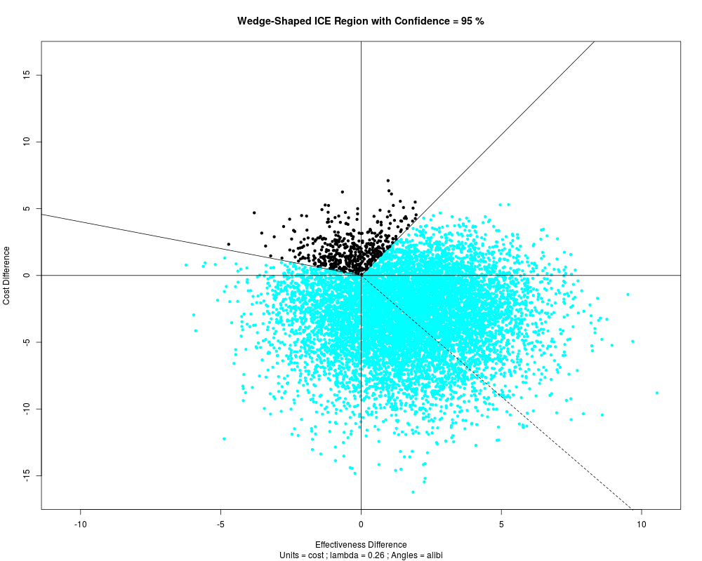
> dpwdg <- ICEwedge(dpunc)

> dpwdg

ICEwedge: Incremental Cost-Effectiveness Bootstrap Confidence Wedge...

Shadow Price of Health, lambda = 0.26
Shadow Price of Health Multiplier, lfact = 1
ICE Differences in both Cost and Effectiveness expressed in cost units.
ICE Angle of the Observed Outcome = -16.107
ICE Ratio of the Observed Outcome = -1.812
Count-Outwards  Central ICE Angle Order Statistic = 4859 of 10000
Counter-Clockwise Upper ICE Angle Order Statistic = 9609
Counter-Clockwise Upper ICE Angle = 111.167
Counter-Clockwise Upper ICE Ratio = 2.26375
    Clockwise     Lower ICE Angle Order Statistic = 109
    Clockwise     Lower ICE Angle = -156.873
    Clockwise     Lower ICE Ratio = -0.40144
ICE Angle Computation Perspective = alibi
Confidence Wedge Subtended ICE Polar Angle = 268.039


> opar <- par(ask = dev.interactive(orNone = TRUE))

> # Click within graphics window to display the Bootstrap 95% Confidence Wedge...
> plot(dpwdg)

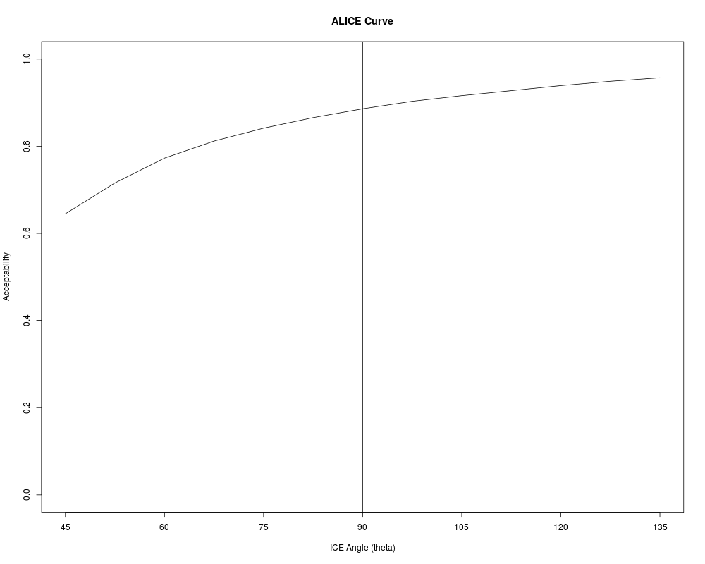
> # Computing VAGR Acceptability and ALICE Curves...
> dpacc <- ICEalice(dpwdg)

> plot(dpacc)

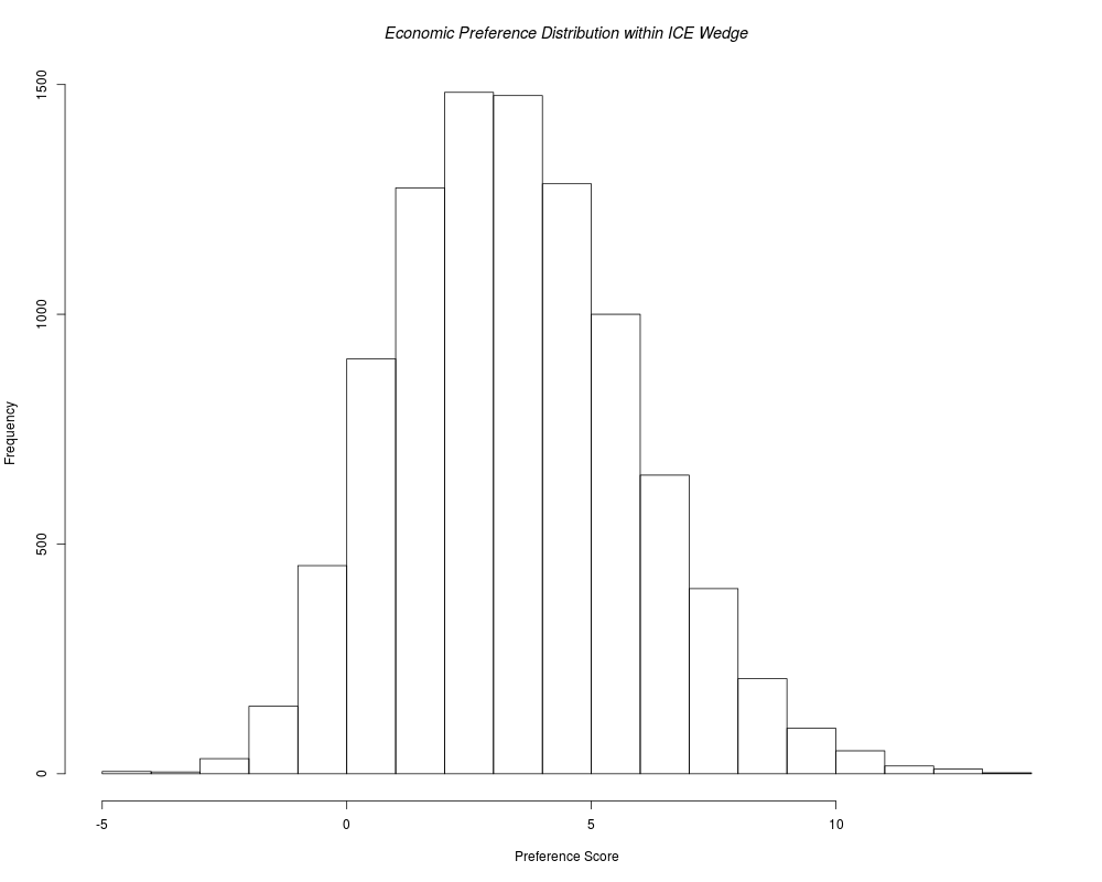
> # Color Interior of Confidence Wedge with LINEAR Economic Preferences...
> dpcol <- ICEcolor(dpwdg, gamma=1)

> plot(dpcol)

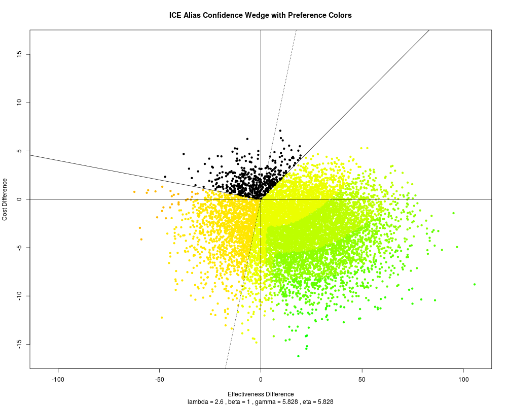
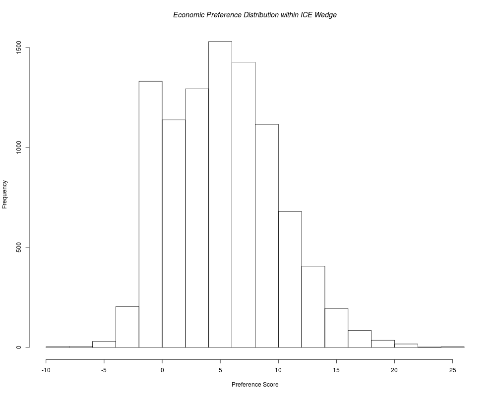
> # Increase Lambda and Recolor Confidence Wedge with NON-Linear Preferences...
> dpcol <- ICEcolor(dpwdg, lfact=10)

> plot(dpcol)

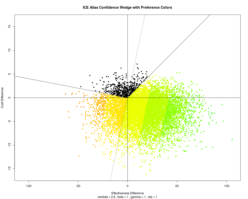
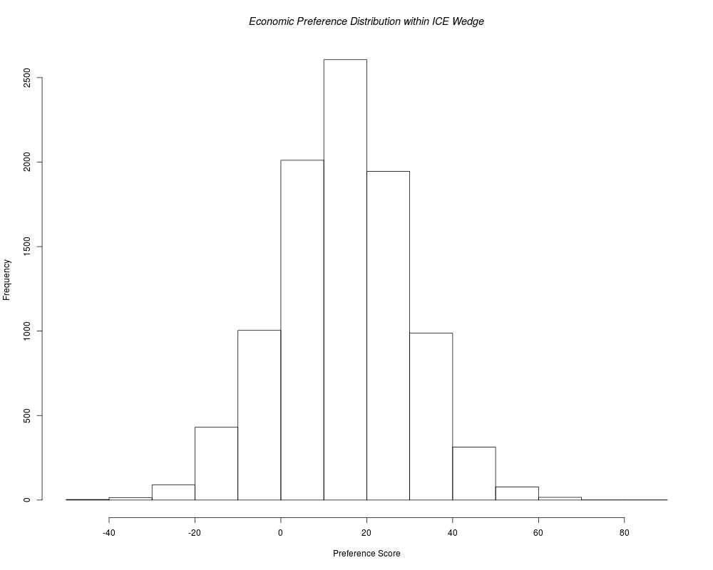
> # Decrease Lambda and Recolor Confidence Wedge with LINEAR Preferences...
> dpcol <- ICEcolor(dpwdg, lfact=10, gamma=1)

> plot(dpcol)

> par(opar)
> 
> 
> 
> 
> 
> dev.off()
null device 
          1 
>