Data for the High Uncertainty numerical example of Obenchain et al. (2005)

Description

The data are from two arms of a double-blind clinical trial in which 91 patients were randomized to the SNRI duloxetine 80 mg/d (40 mg BID) and 87 patients were randomized to the SSRI paroxetine 20 mg/d for treatment of major depressive disorder (MDD). Missing-data- imputation and sensitivity-analyses were needed to make meaningful cost-effectiveness comparisons in this study.

Usage

data(dulxparx)

Format

A data frame of 3 variables on 178 patients; no NAs.

idb

This measure of overall effectiveness is integrated decrease in HAMD-17 score from baseline to endpoint, Hamilton (1967). This is a (signed) area-under-the-curve measure with larger values more favorable. Missing values were imputed via the MMRM models reported in Goldstein et al. (2004).

ru

Patient self-reported health-care resource utilization above and beyond that provided within study protocol was collected using the Resource Utilization Survey, Copley-Merriman et al. (1992), with published 1998 dollars-per-unit costs, Schoenbaum et al. (2001), rounded to the nearest 50 dollars. Dollars/week were then calculated by multiplying (total accumulated cost) for a patient by 7 and dividing by the (total days of cost accumulation) for that patient. For patients who discontinued early, this is Average-Value-Carried-Forward imputation.

dulx

Treatment indicator variable. dulx = 1 implies receipt of duloxetine 80 mg/d (40 mg BID). dulx = 0 implies receipt of paroxetine 20 mg/d.

References

Copley-Merriman C, Egbuonu-Davis L, Kotsanos JG, Conforti P, Franson T, Gordon G. Clinical economics: a method for prospective health resource data collection. Pharmacoeconomics 1992; 1(5): 370–376.

Goldstein DJ, Lu Y, Detke MJ, Wiltse C, Mallincrodt C, Demitrack MA. Duloxetine in the treatment of depression - A double-blind, placebo-controlled comparison with paroxetine. J Clin Psychopharmacol 2004; 24: 389–399.

Hamilton M. Development of a rating scale for primary depressive illness. British Journal of Social and Clinical Psychology 1967; 6: 278–296.

Obenchain RL, Robinson RL, Swindle RW. Cost-effectiveness inferences from bootstrap quadrant confidence levels: three degrees of dominance. J Biopharm Stat 2005; 15(3): 419–436.

Obenchain RL. ICEinR.pdf Vignette-like documentation for ICEinfer stored in the R library/ICEinfer/doc folder. 2009; 30 pages.

Schoenbaum M, Unutzer J, Sherbourne C, Duan N, Rubenstein LV, Miranda J, Meredith LS, Carney MF, Wells K. Cost-effectiveness of practice-initiated quality improvement for depression: results of a randomized controlled trial. JAMA 2001; 286(11): 1325–1330.

Examples

    # Demo of ICEinfer functionality on the dulxparx dataset...
    demo(dulxparx)

Results

R version 3.3.1 (2016-06-21) -- "Bug in Your Hair"
Copyright (C) 2016 The R Foundation for Statistical Computing
Platform: x86_64-pc-linux-gnu (64-bit)

R is free software and comes with ABSOLUTELY NO WARRANTY.
You are welcome to redistribute it under certain conditions.
Type 'license()' or 'licence()' for distribution details.

R is a collaborative project with many contributors.
Type 'contributors()' for more information and
'citation()' on how to cite R or R packages in publications.

Type 'demo()' for some demos, 'help()' for on-line help, or
'help.start()' for an HTML browser interface to help.
Type 'q()' to quit R.

> library(ICEinfer)
Loading required package: lattice
> png(filename="/home/ddbj/snapshot/RGM3/R_CC/result/ICEinfer/dulxparx.Rd_%03d_medium.png", width=480, height=480)
> ### Name: dulxparx
> ### Title: Data for the High Uncertainty numerical example of Obenchain et
> ###   al. (2005)
> ### Aliases: dulxparx
> ### Keywords: datasets
> 
> ### ** Examples
> 
>     # Demo of ICEinfer functionality on the dulxparx dataset...
>     demo(dulxparx)


	demo(dulxparx)
	---- ~~~~~~~~

> require(ICEinfer)

> # input the dulxparx data of Obenchain et al. (2000).
> data(dulxparx)

> # Effectiveness = idb, Cost = ru, trtm = dulx where
> # dulx = 1 ==> Duloxetine treatment and dulx = 0 ==> Paroxetine treatment
> #
> # Display of Lambda => Shadow Price Summary Statistics...
> ICEscale(dulxparx, dulx, idb, ru)

Incremental Cost-Effectiveness (ICE) Lambda Scaling Statistics

Specified Value of Lambda   = 1
Cost and Effe Differences are both expressed in cost units

Effectiveness variable Name = idb
     Cost     variable Name = ru
  Treatment   factor   Name = dulx
New treatment level is = 1 and Standard level is = 0 

Observed  Treatment Diff = 6.152
Std. Error of Trtm Diff  = 8.186 

Observed Cost Difference = -2.899
Std. Error of Cost Diff  = 3.096 

Observed  ICE  Ratio     = -0.471 

Statistical Shadow Price = 0.378
Power-of-Ten Shadow Price= 1 


> ICEscale(dulxparx, dulx, idb, ru, lambda=0.26)

Incremental Cost-Effectiveness (ICE) Lambda Scaling Statistics

Specified Value of Lambda   = 0.26
Cost and Effe Differences are both expressed in cost units

Effectiveness variable Name = idb
     Cost     variable Name = ru
  Treatment   factor   Name = dulx
New treatment level is = 1 and Standard level is = 0 

Observed  Treatment Diff = 1.6
Std. Error of Trtm Diff  = 2.128 

Observed Cost Difference = -2.899
Std. Error of Cost Diff  = 3.096 

Observed  ICE  Ratio     = -1.812 

Statistical Shadow Price = 1.455
Power-of-Ten Shadow Price= 1 


> # Bootstrap ICE Uncertainty calculations can be time consuming...
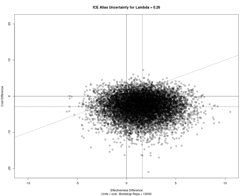
> dpunc <- ICEuncrt(dulxparx, dulx, idb, ru, R = 10000, lambda=0.26)

> dpunc

Incremental Cost-Effectiveness (ICE) Bivariate Bootstrap Uncertainty

Shadow Price = Lambda = 0.26
Bootstrap Replications, R = 10000
Effectiveness variable Name = idb
     Cost     variable Name = ru
  Treatment   factor   Name = dulx
New treatment level is = 1 and Standard level is = 0 

Cost and Effe Differences are both expressed in cost units

Observed  Treatment Diff = 1.6
Mean Bootstrap Trtm Diff = 1.59 

Observed Cost Difference = -2.899
Mean Bootstrap Cost Diff = -2.905 


> # Display the Bootstrap ICE Uncertainty Distribution...
> plot(dpunc)

Incremental Cost-Effectiveness (ICE) Bivariate Bootstrap Uncertainty

Shadow Price = Lambda = 0.26
Bootstrap Replications, R = 10000
Effectiveness variable Name = idb
     Cost     variable Name = ru
  Treatment   factor   Name = dulx
New treatment level is = 1 and Standard level is = 0 

Cost and Effe Differences are both expressed in cost units

Observed  Treatment Diff = 1.6
Mean Bootstrap Trtm Diff = 1.59 

Observed Cost Difference = -2.899
Mean Bootstrap Cost Diff = -2.905 


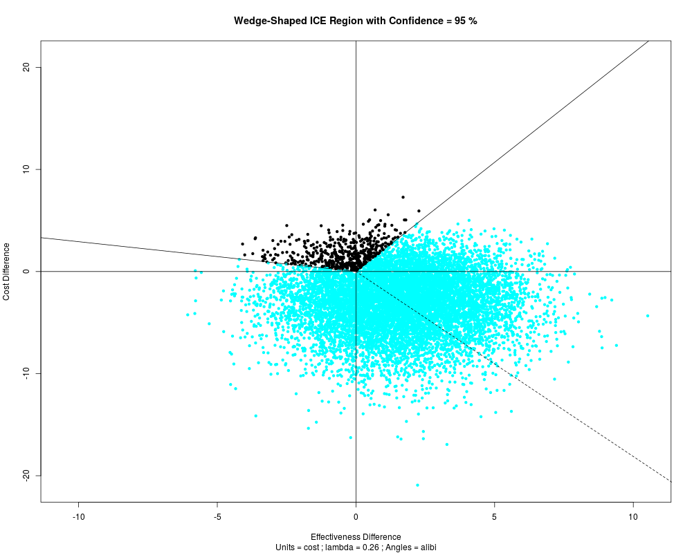
> dpwdg <- ICEwedge(dpunc)

> dpwdg

ICEwedge: Incremental Cost-Effectiveness Bootstrap Confidence Wedge...

Shadow Price of Health, lambda = 0.26
Shadow Price of Health Multiplier, lfact = 1
ICE Differences in both Cost and Effectiveness expressed in cost units.
ICE Angle of the Observed Outcome = -16.107
ICE Ratio of the Observed Outcome = -1.812
Count-Outwards  Central ICE Angle Order Statistic = 4874 of 10000
Counter-Clockwise Upper ICE Angle Order Statistic = 9624
Counter-Clockwise Upper ICE Angle = 111.663
Counter-Clockwise Upper ICE Ratio = 2.31791
    Clockwise     Lower ICE Angle Order Statistic = 124
    Clockwise     Lower ICE Angle = -149.639
    Clockwise     Lower ICE Ratio = -0.26121
ICE Angle Computation Perspective = alibi
Confidence Wedge Subtended ICE Polar Angle = 261.303


> opar <- par(ask = dev.interactive(orNone = TRUE))

> # Click within graphics window to display the Bootstrap 95% Confidence Wedge...
> plot(dpwdg)

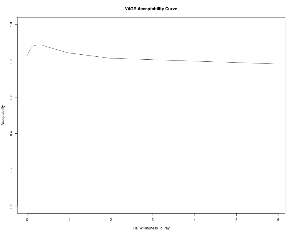
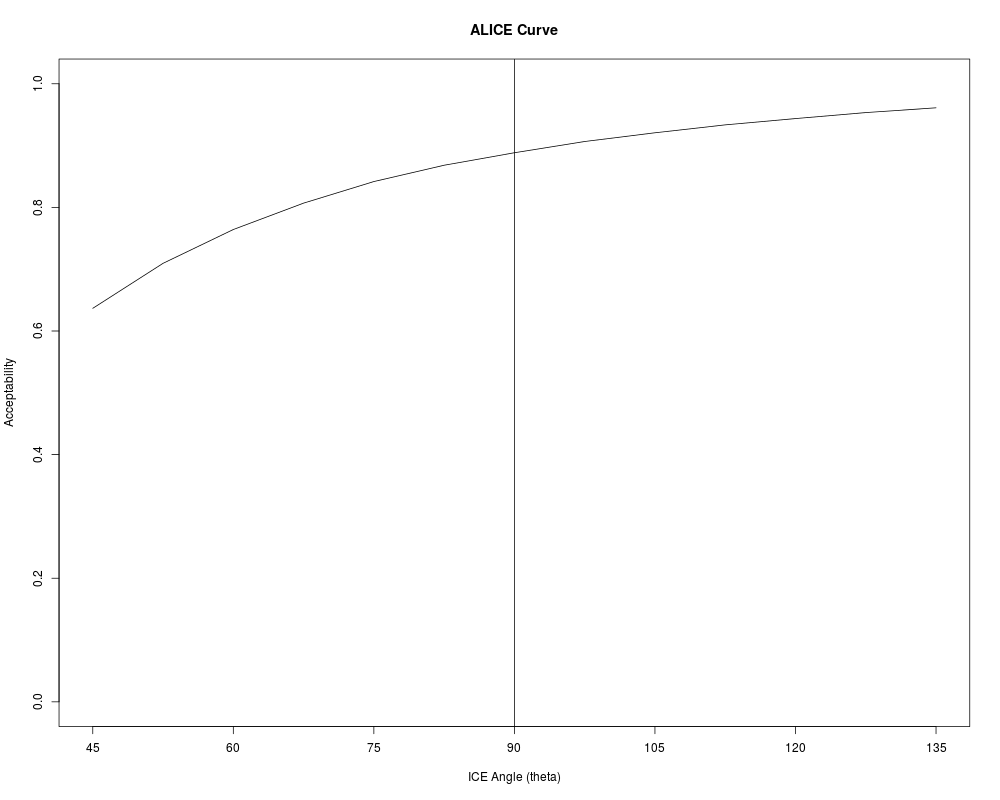
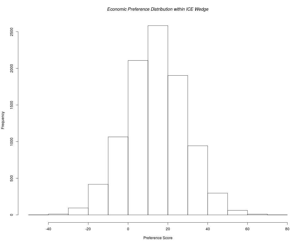
> # Computing VAGR Acceptability and ALICE Curves...
> dpacc <- ICEalice(dpwdg)

> plot(dpacc)

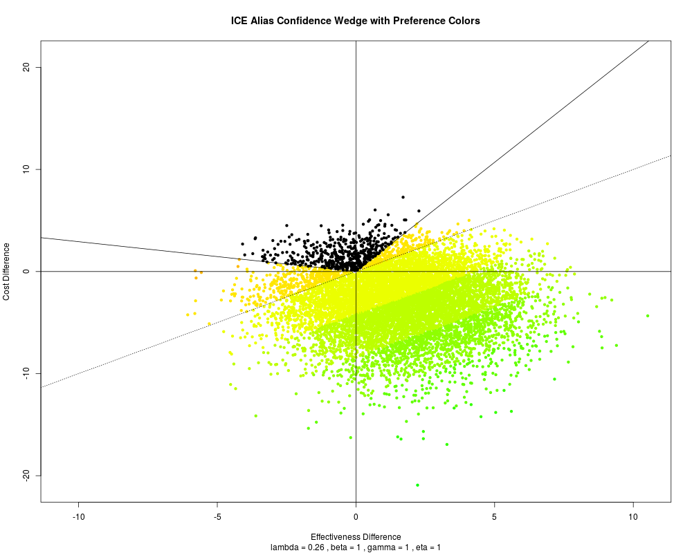
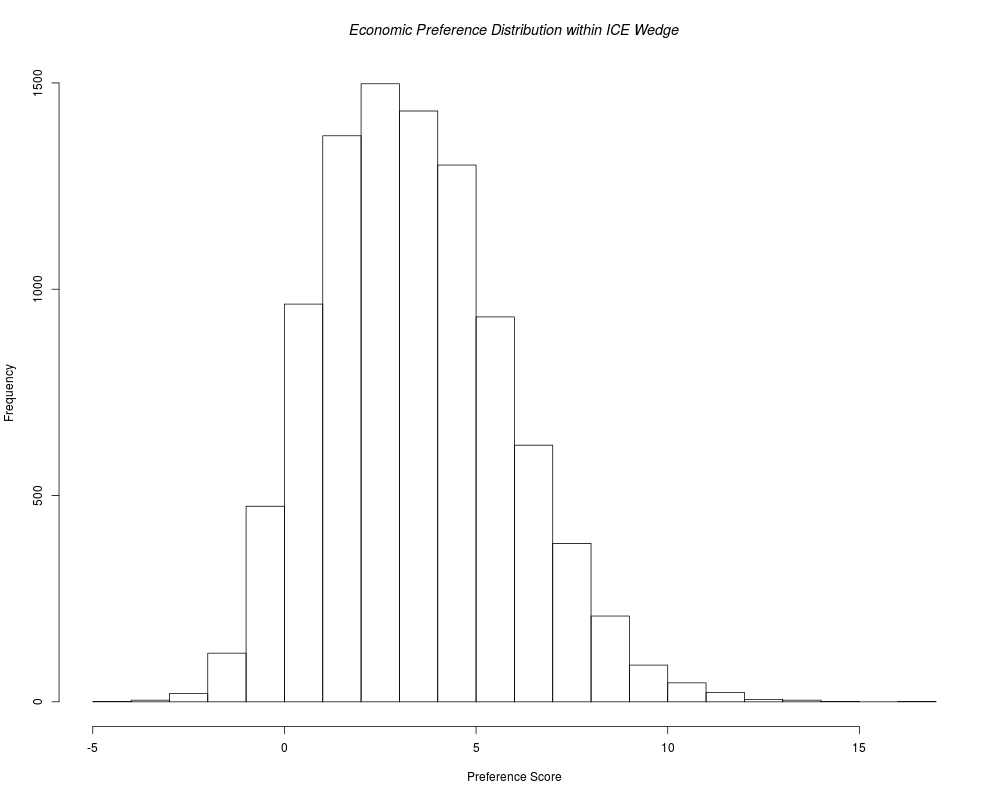
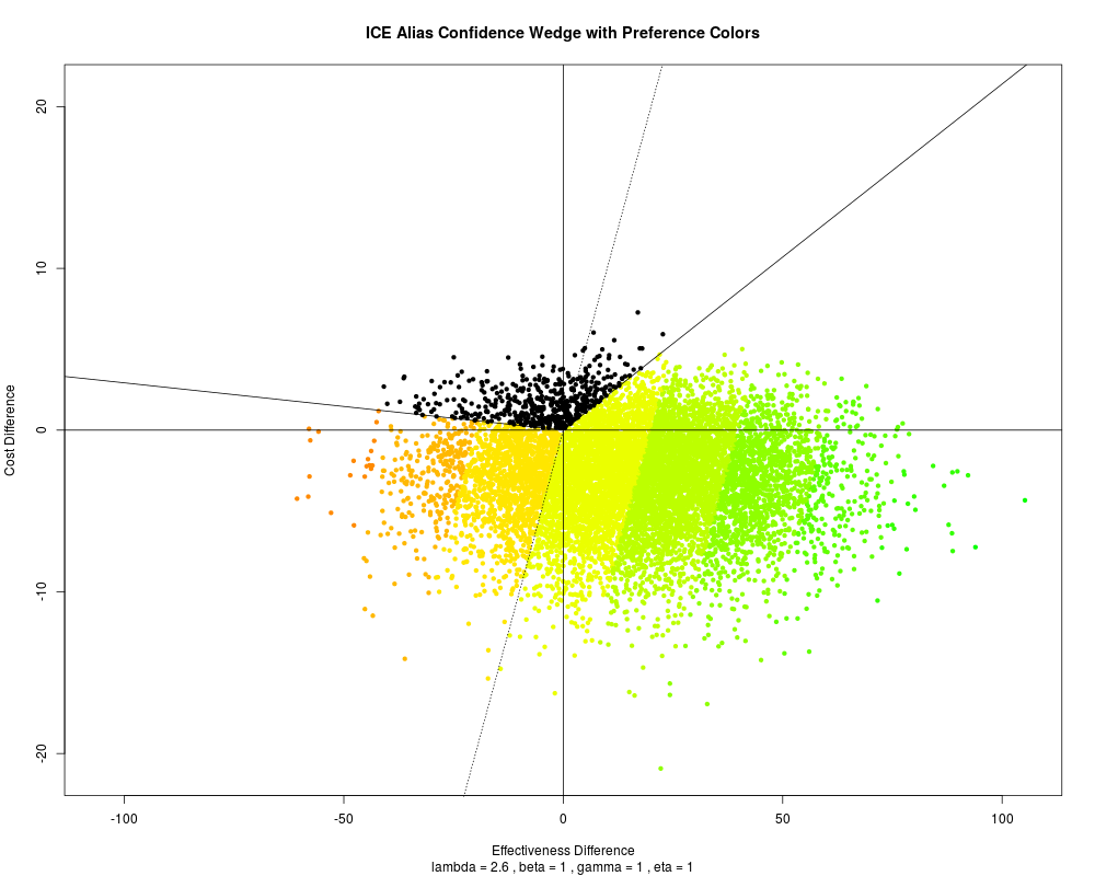
> # Color Interior of Confidence Wedge with LINEAR Economic Preferences...
> dpcol <- ICEcolor(dpwdg, gamma=1)

> plot(dpcol)

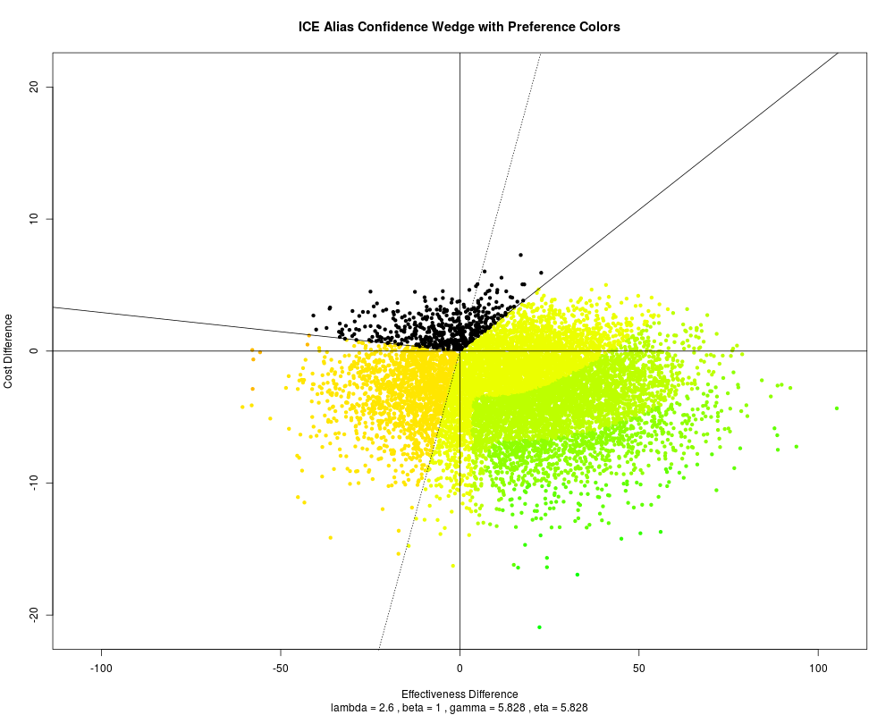
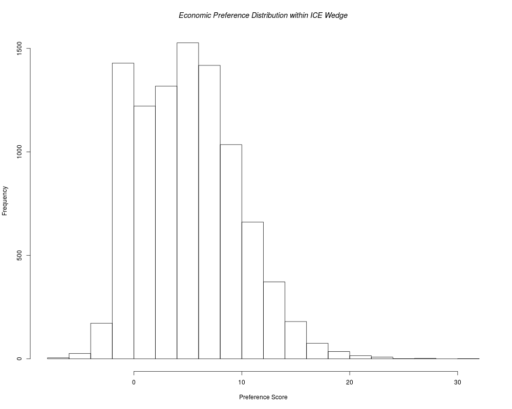
> # Increase Lambda and Recolor Confidence Wedge with NON-Linear Preferences...
> dpcol <- ICEcolor(dpwdg, lfact=10)

> plot(dpcol)

> # Decrease Lambda and Recolor Confidence Wedge with LINEAR Preferences...
> dpcol <- ICEcolor(dpwdg, lfact=10, gamma=1)

> plot(dpcol)

> par(opar)
> 
> 
> 
> 
> 
> dev.off()
null device 
          1 
>