Data from a double-blind clinical trial comparing fluoxetine plus pindolol with fluoxetine alone

Description

These data are from a Spanish double-blind clinical trial in which 55 patients were randomized to fluoxetine (an SSRI) plus pindolol (a Beta Blocker) and 56 patients were randomized to fluoxetine plus placebo for treatment of major depressive disorder (MDD), Sacristan et al. (2000).

Usage

data(fluoxpin)

Format

A data frame of 3 variables on 111 patients; no NAs.

respond

Patients are considered to have responded to treatment when a 50% or greater decrease in HAMD-17 total score occurred between baseline and end-point (at day 42), with no more than 10% additional variation between intermediate visits.

cost

Resource utilization was prospectively collected alongside the clinical trial. Patients and caregivers were interviewed by the researcher concerning all resources consumed during the study period. Resources dictated by the protocol were not counted. Costs are expressed in Pesetas (Pts.) at 1996 prices (1 Dollar = 145 Pts.) Observed differences in average direct medical costs were mainly due to hospitalizations within the FlxPin = 0 group.

flxpin

Treatment indicator variable. FlxPin = 1 implies receipt of fluoxetine 20 mg/day plus pindolol 7.5 mg/day (2.5 mg tid). FlxPin = 0 implies receipt of fluoxetine 20 mg/day plus placebo (tid).

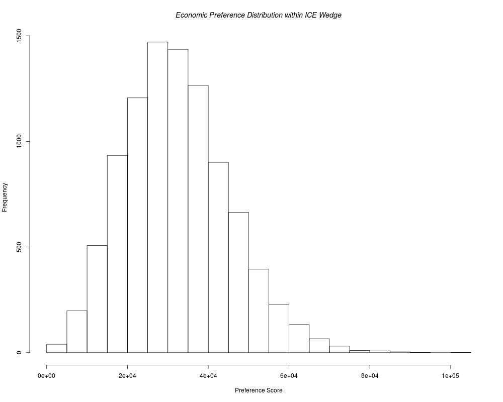
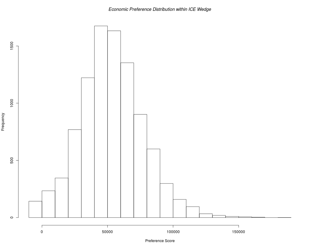
Details

Since both samples are rather small (55 and 56 patients) here and the Effectiveness variable, respond, is binary, this example illustrates how the Law of Large Numbers can fail to apply to ICE inferences. Specifically, the bootstrap distribution of sample differences between AVERAGES appears to be quite different from bivariate normal in three ways: (i) The Bootstrap Distribution of ICE Uncertainty appears to consist of vertical stripes because the horizontal variable is discrete here while the vertical variable is continuous. (ii) The Bootstrap Distribution of cost differences appears to end somewhat abruptly near the horizontal axis at DeltaCost = 0, rather than have a long upwards tail like its downwards tail. (iii) The equal density contours of the bivariate Bootstrap Distribution appear to NOT be elliptical. This third point can be dramaticaly illustrated by computing the Owen Empirical Likelihood contour that passes through the origin of the ICE plane.

References

Hamilton M. Development of a rating scale for primary depressive illness. British Journal of Social and Clinical Psychology 1967; 6: 278–296.

Sacristan JA, Obenchain RL. Reporting cost-effectiveness analyses with confidence. JAMA 1997; 277: 375.

Obenchain RL, Sacristan JA. In reply to: The negative side of cost-effectiveness ratios. JAMA 1997; 277: 1931–1933.

Sacristan JA, Gilaberte I, Boto B, Buesching DP, Obenchain RL, Demitrack M, Perez Sola V, Alvarez E, and Artigas F. Cost-effectiveness of fluoxetine plus pindolol in patients with major depressive disorder: results from a randomized, double blind clinical trial. Int Clin Psychopharmacol 2000; 15: 107–113.

Obenchain RL. ICEinR.pdf Vignette-like documentation for ICEinfer stored in the R library/ICEinfer/doc folder. 2009; 30 pages.

Owen AB. Empirical Likelihood New York: Chapman and Hall/CRC. 2001.

Examples

    # Demo of ICEinfer functionality on the fluoxpin dataset...
    demo(fluoxpin)

Results

R version 3.3.1 (2016-06-21) -- "Bug in Your Hair"
Copyright (C) 2016 The R Foundation for Statistical Computing
Platform: x86_64-pc-linux-gnu (64-bit)

R is free software and comes with ABSOLUTELY NO WARRANTY.
You are welcome to redistribute it under certain conditions.
Type 'license()' or 'licence()' for distribution details.

R is a collaborative project with many contributors.
Type 'contributors()' for more information and
'citation()' on how to cite R or R packages in publications.

Type 'demo()' for some demos, 'help()' for on-line help, or
'help.start()' for an HTML browser interface to help.
Type 'q()' to quit R.

> library(ICEinfer)
Loading required package: lattice
> png(filename="/home/ddbj/snapshot/RGM3/R_CC/result/ICEinfer/fluoxpin.Rd_%03d_medium.png", width=480, height=480)
> ### Name: fluoxpin
> ### Title: Data from a double-blind clinical trial comparing fluoxetine
> ###   plus pindolol with fluoxetine alone
> ### Aliases: fluoxpin
> ### Keywords: datasets
> 
> ### ** Examples
> 
>     # Demo of ICEinfer functionality on the fluoxpin dataset...
>     demo(fluoxpin)


	demo(fluoxpin)
	---- ~~~~~~~~

> require(ICEinfer)

> # input the fluoxpin data of Sacristan et al. (2000).
> data(fluoxpin)

> # Effectiveness = respond, Cost = cost, trtm = flxpin where
> # flxpin = 1 ==> fluoxetine plus pindolol and flxpin = 0 ==> fluoxetine alone
> 
> cat("\n Display of Lambda => Shadow Price Summary Statistics...\n")

 Display of Lambda => Shadow Price Summary Statistics...

> ICEscale(fluoxpin, flxpin, respond, cost)

Incremental Cost-Effectiveness (ICE) Lambda Scaling Statistics

Specified Value of Lambda   = 1
Cost and Effe Differences are both expressed in cost units

Effectiveness variable Name = respond
     Cost     variable Name = cost
  Treatment   factor   Name = flxpin
New treatment level is = 1 and Standard level is = 0 

Observed  Treatment Diff = 0.156
Std. Error of Trtm Diff  = 0.089 

Observed Cost Difference = -29361.751
Std. Error of Cost Diff  = 15438.192 

Observed  ICE  Ratio     = -188012.873 

Statistical Shadow Price = 173534.734
Power-of-Ten Shadow Price= 1e+05 


> ICEscale(fluoxpin, flxpin, respond, cost, lambda=100000)

Incremental Cost-Effectiveness (ICE) Lambda Scaling Statistics

Specified Value of Lambda   = 1e+05
Cost and Effe Differences are both expressed in cost units

Effectiveness variable Name = respond
     Cost     variable Name = cost
  Treatment   factor   Name = flxpin
New treatment level is = 1 and Standard level is = 0 

Observed  Treatment Diff = 15616.883
Std. Error of Trtm Diff  = 8896.312 

Observed Cost Difference = -29361.751
Std. Error of Cost Diff  = 15438.192 

Observed  ICE  Ratio     = -1.88 

Statistical Shadow Price = 1.735
Power-of-Ten Shadow Price= 1 


> cat("\nBootstrap ICE Uncertainty calculations can be lengthy...\n")

Bootstrap ICE Uncertainty calculations can be lengthy...

> fpunc <<- ICEuncrt(fluoxpin, flxpin, respond, cost, R = 10000, lambda=100000)

> fpunc

Incremental Cost-Effectiveness (ICE) Bivariate Bootstrap Uncertainty

Shadow Price = Lambda = 1e+05
Bootstrap Replications, R = 10000
Effectiveness variable Name = respond
     Cost     variable Name = cost
  Treatment   factor   Name = flxpin
New treatment level is = 1 and Standard level is = 0 

Cost and Effe Differences are both expressed in cost units

Observed  Treatment Diff = 15616.883
Mean Bootstrap Trtm Diff = 15656.321 

Observed Cost Difference = -29361.751
Mean Bootstrap Cost Diff = -29389.906 


> cat("\nDisplay the Bootstrap ICE Uncertainty Distribution...\n")

Display the Bootstrap ICE Uncertainty Distribution...

> plot(fpunc)

Incremental Cost-Effectiveness (ICE) Bivariate Bootstrap Uncertainty

Shadow Price = Lambda = 1e+05
Bootstrap Replications, R = 10000
Effectiveness variable Name = respond
     Cost     variable Name = cost
  Treatment   factor   Name = flxpin
New treatment level is = 1 and Standard level is = 0 

Cost and Effe Differences are both expressed in cost units

Observed  Treatment Diff = 15616.883
Mean Bootstrap Trtm Diff = 15656.321 

Observed Cost Difference = -29361.751
Mean Bootstrap Cost Diff = -29389.906 


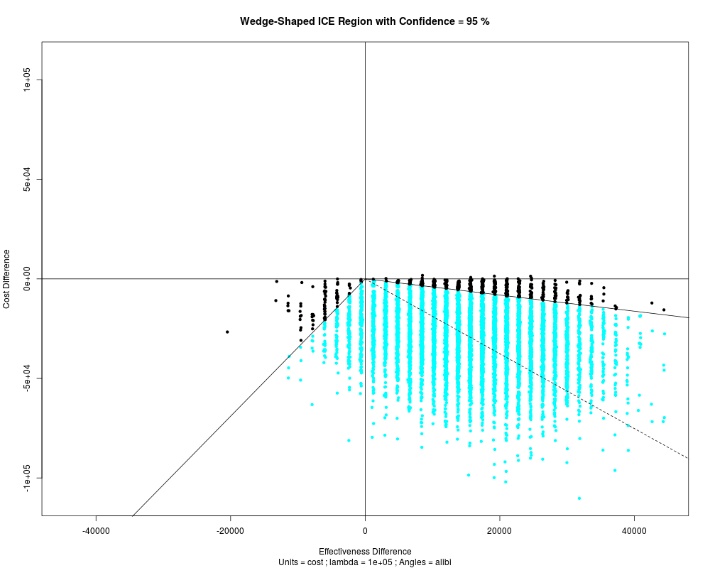
> fpwdg <- ICEwedge(fpunc)

> fpwdg

ICEwedge: Incremental Cost-Effectiveness Bootstrap Confidence Wedge...

Shadow Price of Health, lambda = 1e+05
Shadow Price of Health Multiplier, lfact = 1
ICE Differences in both Cost and Effectiveness expressed in cost units.
ICE Angle of the Observed Outcome = -16.992
ICE Ratio of the Observed Outcome = -1.88013
Count-Outwards  Central ICE Angle Order Statistic = 4893 of 10000
Counter-Clockwise Upper ICE Angle Order Statistic = 9643
Counter-Clockwise Upper ICE Angle = 24.015
Counter-Clockwise Upper ICE Ratio = -0.38357
    Clockwise     Lower ICE Angle Order Statistic = 143
    Clockwise     Lower ICE Angle = -57.123
    Clockwise     Lower ICE Ratio = 4.65532
ICE Angle Computation Perspective = alibi
Confidence Wedge Subtended ICE Polar Angle = 81.138


> opar <- par(ask = dev.interactive(orNone = TRUE))

> cat("\nClick within graphics window to display the Bootstrap 95% Confidence Wedge...\n")

Click within graphics window to display the Bootstrap 95% Confidence Wedge...

> plot(fpwdg)

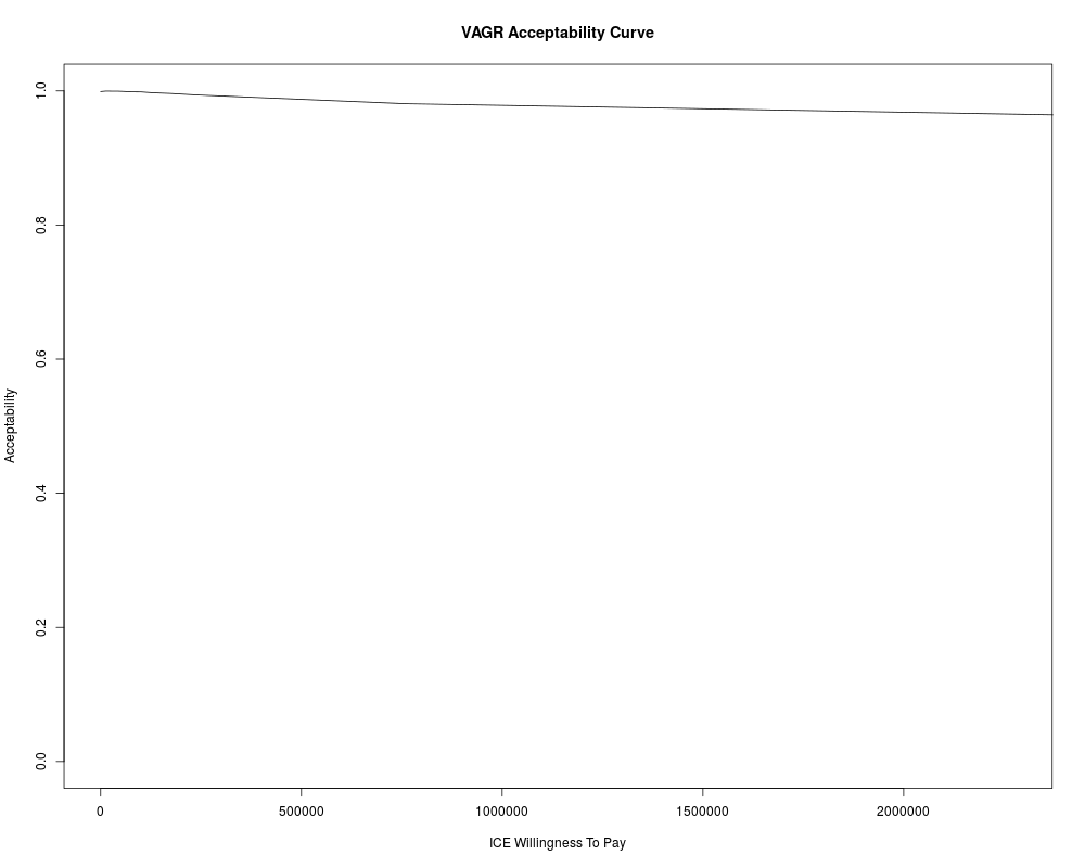
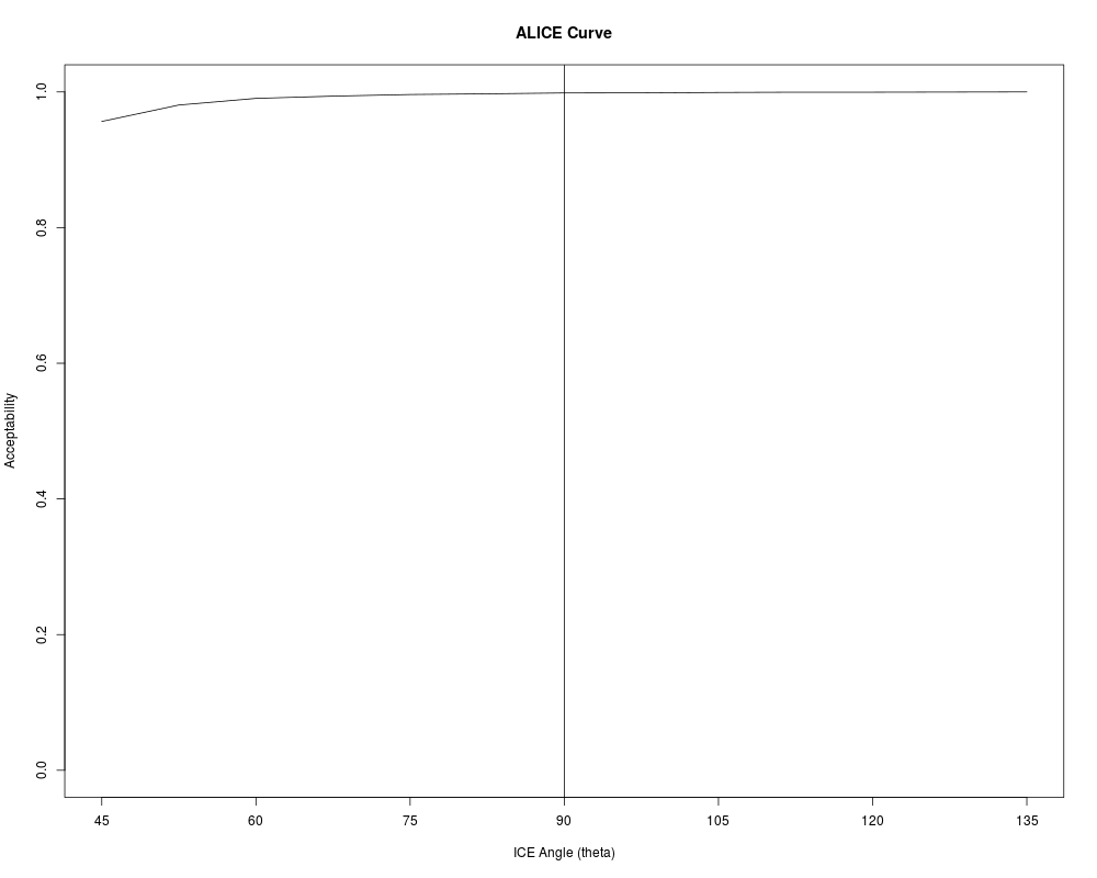
> cat("\nComputing VAGR Acceptability and ALICE Curves...\n")

Computing VAGR Acceptability and ALICE Curves...

> fpacc <- ICEalice(fpwdg)

> plot(fpacc)

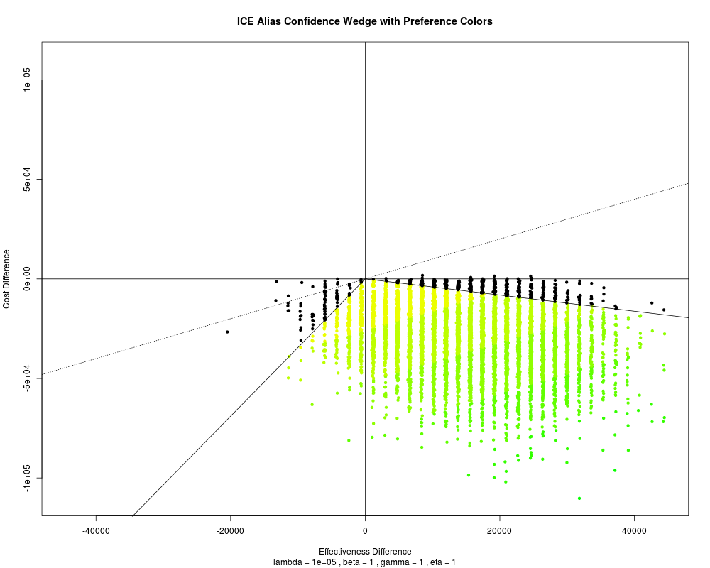
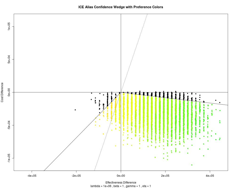
> cat("\nColor Interior of Confidence Wedge with LINEAR Economic Preferences...\n")

Color Interior of Confidence Wedge with LINEAR Economic Preferences...

> fpcol <- ICEcolor(fpwdg, gamma=1)

> plot(fpcol)

> cat("\nIncrease Lambda and Recolor Confidence Wedge with NON-Linear Preferences...\n")

Increase Lambda and Recolor Confidence Wedge with NON-Linear Preferences...

> fpcol <- ICEcolor(fpwdg, lfact=10)

> plot(fpcol)

> cat("\nDecrease Lambda and Recolor Confidence Wedge with LINEAR Preferences...\n")

Decrease Lambda and Recolor Confidence Wedge with LINEAR Preferences...

> fpcol <- ICEcolor(fpwdg, lfact=10, gamma=1)

> plot(fpcol)

> par(opar)
> 
> 
> 
> 
> 
> dev.off()
null device 
          1 
>