Cost-Effectiveness data for 1242 MDD patients from Marketscan(SM) claims database

Description

In 1990-1992, the Marketscan(SM) database included medical and pharmacy claims for approximately 700,000 individuals whose health insurance was provided by large corporations throughout the United States. Outcomes for 1242 patients treated with either fluoxetine (SSRI) or with a TCA / HCA for major depressive disorder (MDD) were discussed in Croghan et al. (1996) and Obenchain et al. (1997). All 1242 patients were continuously enrolled for at least 4 months prior to their initial antidepressant prescription and for the following 12 months.

Usage

data(fluoxtca)

Format

A data frame of 3 variables on 1242 patients; no NAs.

stable

stable = 1 indicates that the patient remained on his/her initial antidepressant medication for at least six consecutive months.

cost

cost is the Marketscan(SM) 12 month total annual charge for a patient.

fluox

Treatment indicator variable; fluox = 1 indicates receipt of fluoxetine 20 mg/d by 799 patients. fluox = 0 implies receipt of either a tricyclic (TCA) or a heterocyclic (HCA) by 443 patients.

Details

This dataset contains measures of cost and efffectiveness for 799 patients treated with fluoxetine (a Selective Serotonin Reuptake Inhibitor or SSRI), 104 patients treated with a first generation tricyclic, TCA (amitriptyline or imipramine), 250 patients treated with a second generation TCA (desipramine or nortriptyline), and 89 patients treated with trazodone (a heterocyclic, HCA).

References

Croghan TW, Lair TJ, Engelhart L, et al. Effect of antidepressant therapy on health care utilization and costs in primary care. Working paper, Eli Lilly and Company, 1996. (Presented in part at the Association for Health Services Research meeting, Chicago, June 9, 1995.)

Obenchain RL, Melfi CA, Croghan TW, Buesching DP. Bootstrap analyses of cost-effectiveness in antidepressant pharmacotherapy. PharmacoEconomics 1997; 17: 1200–1206.

Obenchain RL. ICEplane: a windows application for incremental cost-effectiveness (ICE) statistical inference. Copyright(c) Pharmaceutical Research and Manufacturers of America (PhRMA.) http://members.iquest.net/~softrx/ Revised 1997–2007.

Obenchain RL. ICEinR.pdf Vignette-like documentation for ICEinfer stored in the R library/ICEinfer/doc folder. 2009; 30 pages.

Sclar DA, Robinson LM, Skaer TL, Legg RF, Nemec NL, Galin RS, Hugher TE, Buesching DP. Antidepressant pharmacotherapy: economic outcomes in a health maintenance organization. Clin Ther 1994; 16: 715–730.

Examples

    # Demo of ICEinfer functionality on the fluoxtca dataset...
    demo(fluoxtca)

Results

R version 3.3.1 (2016-06-21) -- "Bug in Your Hair"
Copyright (C) 2016 The R Foundation for Statistical Computing
Platform: x86_64-pc-linux-gnu (64-bit)

R is free software and comes with ABSOLUTELY NO WARRANTY.
You are welcome to redistribute it under certain conditions.
Type 'license()' or 'licence()' for distribution details.

R is a collaborative project with many contributors.
Type 'contributors()' for more information and
'citation()' on how to cite R or R packages in publications.

Type 'demo()' for some demos, 'help()' for on-line help, or
'help.start()' for an HTML browser interface to help.
Type 'q()' to quit R.

> library(ICEinfer)
Loading required package: lattice
> png(filename="/home/ddbj/snapshot/RGM3/R_CC/result/ICEinfer/fluoxtca.Rd_%03d_medium.png", width=480, height=480)
> ### Name: fluoxtca
> ### Title: Cost-Effectiveness data for 1242 MDD patients from
> ###   Marketscan(SM) claims database
> ### Aliases: fluoxtca
> ### Keywords: datasets
> 
> ### ** Examples
> 
>     # Demo of ICEinfer functionality on the fluoxtca dataset...
>     demo(fluoxtca)


	demo(fluoxtca)
	---- ~~~~~~~~

> require(ICEinfer)

> # input the fluoxtca data of Obenchain et al. (1997).
> data(fluoxtca)

> # Effectiveness = stable, Cost = cost, Trtm = fluox where
> # fluox = 1 ==> fluoxetine treatment and fluox = 0 ==> TCA or HCA
> #
> # Display of Lambda => Shadow Price Summary Statistics...
> 
> ICEscale(fluoxtca, fluox, stable, cost)

Incremental Cost-Effectiveness (ICE) Lambda Scaling Statistics

Specified Value of Lambda   = 1
Cost and Effe Differences are both expressed in cost units

Effectiveness variable Name = stable
     Cost     variable Name = cost
  Treatment   factor   Name = fluox
New treatment level is = 1 and Standard level is = 0 

Observed  Treatment Diff = 0.117
Std. Error of Trtm Diff  = 0.028 

Observed Cost Difference = -192.935
Std. Error of Cost Diff  = 1003.158 

Observed  ICE  Ratio     = -1647.861 

Statistical Shadow Price = 36416.684
Power-of-Ten Shadow Price= 10000 


> ICEscale(fluoxtca, fluox, stable, cost, lambda=10000)

Incremental Cost-Effectiveness (ICE) Lambda Scaling Statistics

Specified Value of Lambda   = 10000
Cost and Effe Differences are both expressed in cost units

Effectiveness variable Name = stable
     Cost     variable Name = cost
  Treatment   factor   Name = fluox
New treatment level is = 1 and Standard level is = 0 

Observed  Treatment Diff = 1170.82
Std. Error of Trtm Diff  = 275.467 

Observed Cost Difference = -192.935
Std. Error of Cost Diff  = 1003.158 

Observed  ICE  Ratio     = -0.165 

Statistical Shadow Price = 3.642
Power-of-Ten Shadow Price= 1 


> # Bootstrap ICE Uncertainty calculations can be lengthy...
> ftunc <- ICEuncrt(fluoxtca, fluox, stable, cost, R = 10000, lambda=10000)

> ftunc

Incremental Cost-Effectiveness (ICE) Bivariate Bootstrap Uncertainty

Shadow Price = Lambda = 10000
Bootstrap Replications, R = 10000
Effectiveness variable Name = stable
     Cost     variable Name = cost
  Treatment   factor   Name = fluox
New treatment level is = 1 and Standard level is = 0 

Cost and Effe Differences are both expressed in cost units

Observed  Treatment Diff = 1170.82
Mean Bootstrap Trtm Diff = 1169.47 

Observed Cost Difference = -192.935
Mean Bootstrap Cost Diff = -200.25 


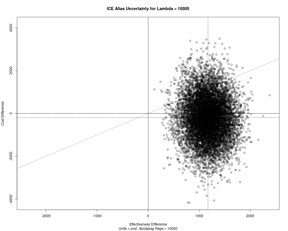
> # Display the Bootstrap ICE Uncertainty Distribution...\n")
> plot(ftunc)

Incremental Cost-Effectiveness (ICE) Bivariate Bootstrap Uncertainty

Shadow Price = Lambda = 10000
Bootstrap Replications, R = 10000
Effectiveness variable Name = stable
     Cost     variable Name = cost
  Treatment   factor   Name = fluox
New treatment level is = 1 and Standard level is = 0 

Cost and Effe Differences are both expressed in cost units

Observed  Treatment Diff = 1170.82
Mean Bootstrap Trtm Diff = 1169.47 

Observed Cost Difference = -192.935
Mean Bootstrap Cost Diff = -200.25 


> ftwdg <- ICEwedge(ftunc)

> ftwdg

ICEwedge: Incremental Cost-Effectiveness Bootstrap Confidence Wedge...

Shadow Price of Health, lambda = 10000
Shadow Price of Health Multiplier, lfact = 1
ICE Differences in both Cost and Effectiveness expressed in cost units.
ICE Angle of the Observed Outcome = 35.643
ICE Ratio of the Observed Outcome = -0.16479
Count-Outwards  Central ICE Angle Order Statistic = 5094 of 10000
Counter-Clockwise Upper ICE Angle Order Statistic = 9844
Counter-Clockwise Upper ICE Angle = 108.728
Counter-Clockwise Upper ICE Ratio = 2.02581
    Clockwise     Lower ICE Angle Order Statistic = 344
    Clockwise     Lower ICE Angle = -16.836
    Clockwise     Lower ICE Ratio = -1.86781
ICE Angle Computation Perspective = alibi
Confidence Wedge Subtended ICE Polar Angle = 125.564


> opar <- par(ask = dev.interactive(orNone = TRUE))

> # Click within graphics window to display the Bootstrap 95% Confidence Wedge...
> plot(ftwdg)

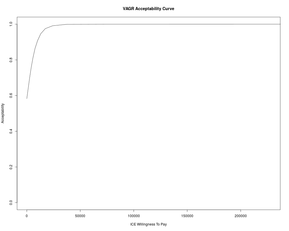
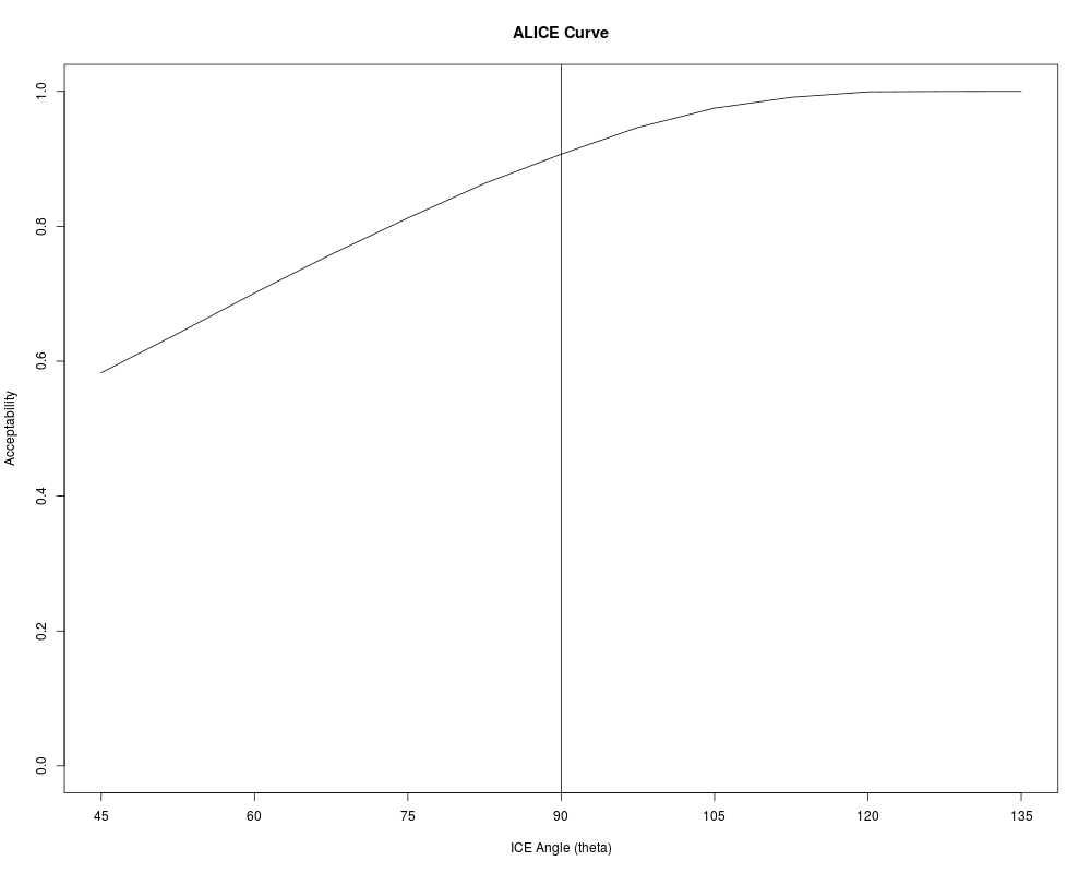
> # Computing VAGR Acceptability and ALICE Curves...\n")
> ftacc <- ICEalice(ftwdg)

> plot(ftacc)

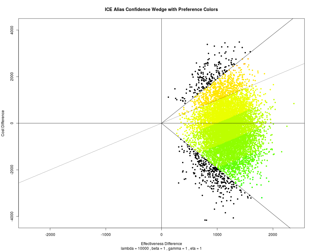
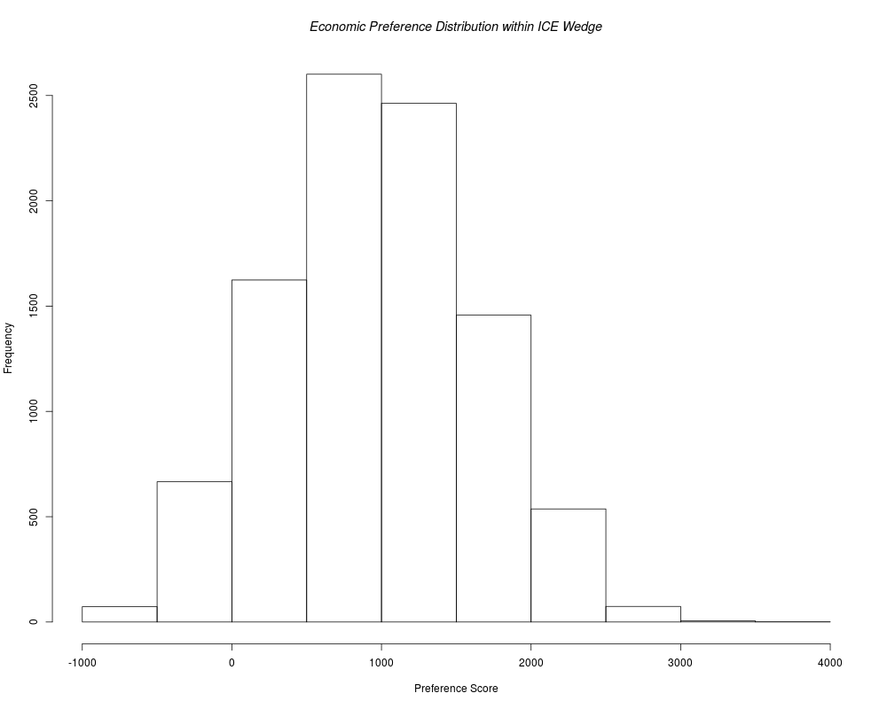
> # Color Interior of Confidence Wedge with LINEAR Economic Preferences...
> ftcol <- ICEcolor(ftwdg, gamma=1)

> plot(ftcol)

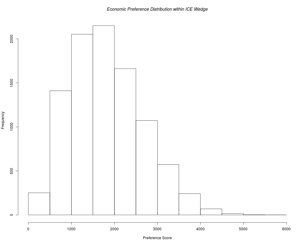
> # Increase Lambda and Recolor Confidence Wedge with NON-Linear Preferences...
> ftcol2 <- ICEcolor(ftwdg, lfact=10)

> plot(ftcol2)

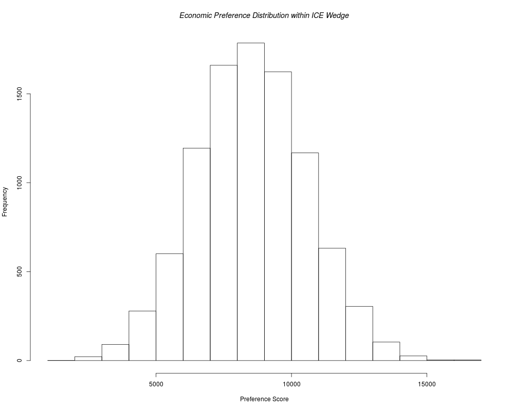
> # Decrease Lambda and Recolor Confidence Wedge with LINEAR Preferences...
> ftcol3 <- ICEcolor(ftwdg, lfact=10, gamma=1)

> plot(ftcol3)

> par(opar)
> 
> 
> 
> 
> 
> dev.off()
null device 
          1 
>