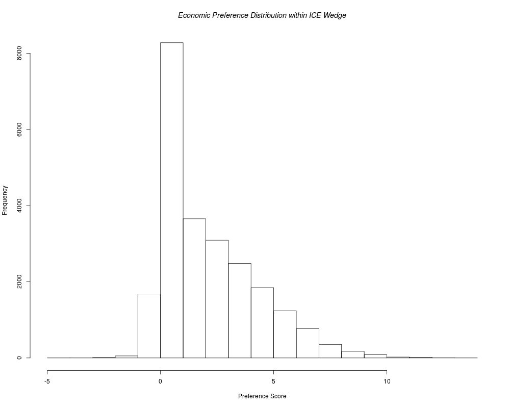
Add Economic Preference Colors to Bootstrap Uncertainty Scatters within a Confidence Wedge

Description

Assuming x is an object of class ICEcolor, the default invocation of plot(x) recolors the default alias display of the points within the bootstrap distribution of ICE uncertainty that are within its statistical confidence wedge. An invocation of the form plot(x, alibi=TRUE) recolors the alibi display. When ready, the user should click within this graphics window to display a Histogram of all the Economic Preference values falling within the ICE Statistical Confidence Wedge.

Usage

  ## S3 method for class 'ICEcolor'
plot(x, alibi = FALSE, ...)

Arguments

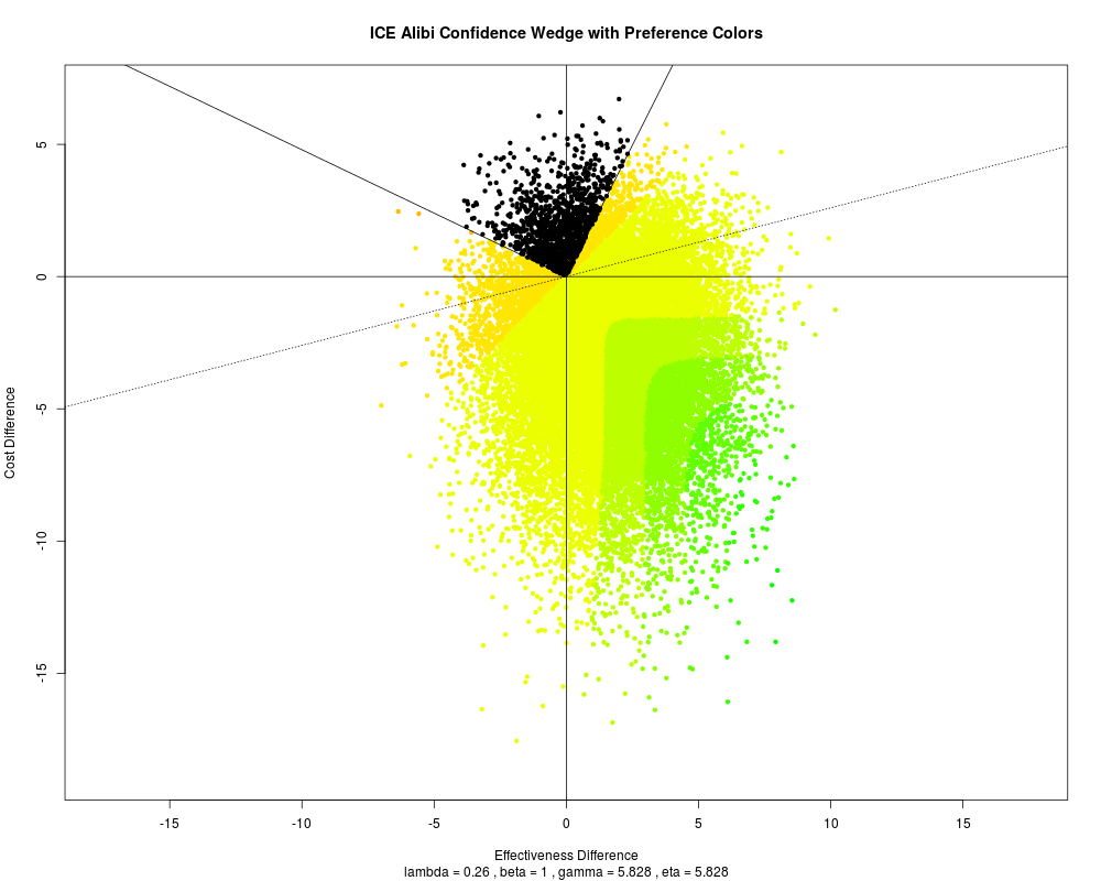
Details

To illustrate the sensitivity of Economic Preferences to choice of lambda, multiple calls are usually made to ICEcolor() for different values of lambda as well as for different choices of the beta and gamma parameters that determine the shape of and spacing between the Indifference Curves of an ICE Preference Map.

The plot() of an object of class ICEcolor displays the Bootstrap Distribution of ICE Uncertainty using small, circular, colored dots (pch = 20). Outcomes outside the Confidence Wedge are displayed in black, while outcomes inside the Wedge are displayed in a rainbow of colors (within the red-tan-yellow-green range) that represent Economic Preferences.

Upper and lower ICE Ray Limits are again displayed as solid black lines, while the Straight Line through the ICE origin that represents lambda is shown as a dashed black line. In an Alias graphic, the slope of this dashed, black line will always be one; however, this dashed line usually does not appear to bisect the North-East and South-West ICE quadrants because DIFFERENT SCALINGS are being used along the horizontal and vertical axes. In an Alibi graphic where the scaling along both axes is the SAME, the slope of this dashed, black line will always be lambda; this dashed line will thus not bisect the North-East and South-West ICE quadrants unless lambda = 1.

Value

NULL

Author(s)

Bob Obenchain <wizbob@att.net>

References

Cook JR, Heyse JF. Use of an angular transformation for ratio estimation in cost-effectiveness analysis. Statistics in Medicine 2000; 19: 2989-3003.

Obenchain RL. Incremental Cost-Effectiveness (ICE) Preference Maps. 2001 JSM Proceedings (Biopharmaceutical Section) on CD-ROM. (10 pages.) Alexandria, VA: American Statistical Association. 2002.

Obenchain RL. ICE Preference Maps: Nonlinear Generalizations of Net Benefit and Acceptability. Health Serv Outcomes Res Method 2008; 8: 31-56. DOI 10.1007/s10742-007-0027-2. Open Access.

See Also

ICEcolor, ICEscale and ICEwedge.

Examples

  data(dpwdg) 
  dpcol <- ICEcolor(dpwdg)
  plot(dpcol)
  plot(dpcol, alibi=TRUE)

Results

R version 3.3.1 (2016-06-21) -- "Bug in Your Hair"
Copyright (C) 2016 The R Foundation for Statistical Computing
Platform: x86_64-pc-linux-gnu (64-bit)

R is free software and comes with ABSOLUTELY NO WARRANTY.
You are welcome to redistribute it under certain conditions.
Type 'license()' or 'licence()' for distribution details.

R is a collaborative project with many contributors.
Type 'contributors()' for more information and
'citation()' on how to cite R or R packages in publications.

Type 'demo()' for some demos, 'help()' for on-line help, or
'help.start()' for an HTML browser interface to help.
Type 'q()' to quit R.

> library(ICEinfer)
Loading required package: lattice
> png(filename="/home/ddbj/snapshot/RGM3/R_CC/result/ICEinfer/plot.ICEcolor.Rd_%03d_medium.png", width=480, height=480)
> ### Name: plot.ICEcolor
> ### Title: Add Economic Preference Colors to Bootstrap Uncertainty Scatters
> ###   within a Confidence Wedge
> ### Aliases: plot.ICEcolor
> ### Keywords: methods hplot
> 
> ### ** Examples
> 
>   data(dpwdg) 
>   dpcol <- ICEcolor(dpwdg)
>   plot(dpcol)
>   plot(dpcol, alibi=TRUE)
> 
> 
> 
> 
> 
> dev.off()
null device 
          1 
>