Modified Procrustes distance

Description

dproc2 computes and returns all the pairwise procrustes distances between genes in a time course experiment, using their expression profile.

Usage

dproc2(x, timepoints = NULL)

Arguments

Details

Each row i of matrix x is arranged in a two column matrix Xi. In Xi, the first column contains the time points and the second column the observed gene expression values (xi1...).

Value

A dist object with distance information.

Author(s)

Itziar Irigoien itziar.irigoien@ehu.es; Konputazio Zientziak eta Adimen Artifiziala, Euskal Herriko Unibertsitatea (UPV-EHU), Donostia, Spain.

Conchita Arenas carenas@ub.edu; Departament d'Estadistica, Universitat de Barcelona, Barcelona, Spain.

References

Irigoien, I. , Vives, S. and Arenas, C. (2011). Microarray Time Course Experiments: Finding Profiles. IEEE/ACM Transactions on Computational Biology and Bioinformatics, 8(2), 464–475.

Gower, J. C. and Dijksterhuis, G. B. (2004) Procrustes Problems. Oxford University Press.

Sibson, R. (1978). Studies in the Robustness of Multidimensional Scaling: Procrustes statistic. Journal of the Royal Statistical Society, Series B, 40, 234–238.

See Also

dist, dmahal, dgower, dcor dbhatta

Examples

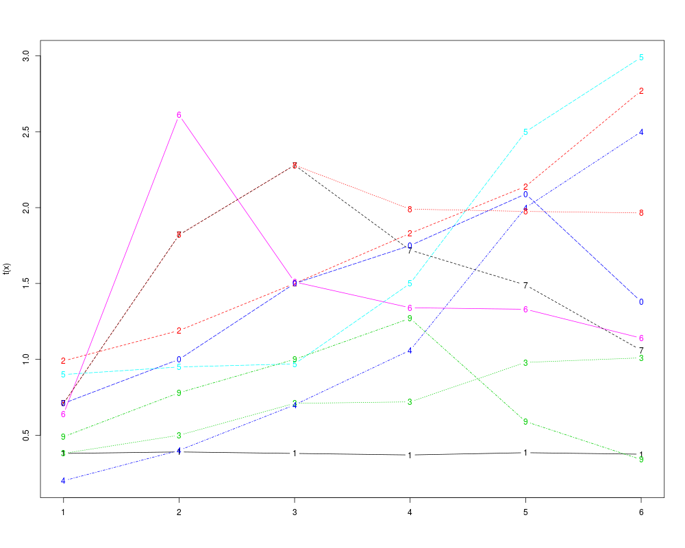
# Given  10  hypothetical time course profiles
# over 6 time points at 1, 2, ..., 6 hours.
x <- matrix(c(0.38, 0.39, 0.38, 0.37, 0.385, 0.375,
              0.99, 1.19, 1.50, 1.83, 2.140, 2.770,
              0.38, 0.50, 0.71, 0.72, 0.980, 1.010,
              0.20, 0.40, 0.70, 1.06, 2.000, 2.500,
              0.90, 0.95, 0.97, 1.50, 2.500, 2.990,
              0.64, 2.61, 1.51, 1.34, 1.330 ,1.140,
              0.71, 1.82, 2.28, 1.72, 1.490, 1.060,
              0.71, 1.82, 2.28, 1.99, 1.975, 1.965,
              0.49, 0.78, 1.00, 1.27, 0.590, 0.340,
              0.71,1.00, 1.50, 1.75, 2.090, 1.380), nrow=10, byrow=TRUE)

# Graphical representation
matplot(t(x), type="b")

# Distance matrix between them
d <- dproc2(x)

Results

R version 3.3.1 (2016-06-21) -- "Bug in Your Hair"
Copyright (C) 2016 The R Foundation for Statistical Computing
Platform: x86_64-pc-linux-gnu (64-bit)

R is free software and comes with ABSOLUTELY NO WARRANTY.
You are welcome to redistribute it under certain conditions.
Type 'license()' or 'licence()' for distribution details.

R is a collaborative project with many contributors.
Type 'contributors()' for more information and
'citation()' on how to cite R or R packages in publications.

Type 'demo()' for some demos, 'help()' for on-line help, or
'help.start()' for an HTML browser interface to help.
Type 'q()' to quit R.

> library(ICGE)
Loading required package: MASS
Loading required package: cluster
> png(filename="/home/ddbj/snapshot/RGM3/R_CC/result/ICGE/dproc2.Rd_%03d_medium.png", width=480, height=480)
> ### Name: dproc2
> ### Title: Modified Procrustes distance
> ### Aliases: dproc2
> ### Keywords: multivariate
> 
> ### ** Examples
> 
> # Given  10  hypothetical time course profiles
> # over 6 time points at 1, 2, ..., 6 hours.
> x <- matrix(c(0.38, 0.39, 0.38, 0.37, 0.385, 0.375,
+               0.99, 1.19, 1.50, 1.83, 2.140, 2.770,
+               0.38, 0.50, 0.71, 0.72, 0.980, 1.010,
+               0.20, 0.40, 0.70, 1.06, 2.000, 2.500,
+               0.90, 0.95, 0.97, 1.50, 2.500, 2.990,
+               0.64, 2.61, 1.51, 1.34, 1.330 ,1.140,
+               0.71, 1.82, 2.28, 1.72, 1.490, 1.060,
+               0.71, 1.82, 2.28, 1.99, 1.975, 1.965,
+               0.49, 0.78, 1.00, 1.27, 0.590, 0.340,
+               0.71,1.00, 1.50, 1.75, 2.090, 1.380), nrow=10, byrow=TRUE)
> 
> # Graphical representation
> matplot(t(x), type="b")
> 
> # Distance matrix between them
> d <- dproc2(x)
> 
> 
> 
> 
> 
> 
> dev.off()
null device 
          1 
>