Two Scatter Matrix ICS Transformation

Description

This function implements the 2 scatter matrix transformation to obtain an invariant coordinate sytem or independent components, depending on the underlying assumptions.

Usage

ics(X, S1 = cov, S2 = cov4, S1args = list(), S2args = list(), 
    stdB = "Z", stdKurt = TRUE, na.action = na.fail)

Arguments

Details

Seeing this function as a tool for data transformation the result is an invariant coordinate selection which can be used for testing and estimation. And if needed the results can be easily retransformed to the original scale. It is possible to use it also for dimension reduction, finding outliers or when searching for clusters in the data. The function can, however, also be used in a modelling framework. In this case it is assumed that the data were created by mixing independent components which have different kurtosis values. If the two scatter matrices used have then the so-called independence property the function can recover the independet components by estimating the unmixing matrix.

By default S1 is the regular covariance matrix cov and S2 the matrix of fourth moments cov4. However those can be replaced with any other scatter matrix the user prefers. The package ICS offers for example also cov4.wt, covAxis, covOrigin or tM and in the ICSNP are for example further scatters as duembgen.shape, tyler.shape, HR.Mest or HP1.shape. But of course also scatters from any other package can be used.

Note that when function names are submitted, the function should return only a scatter matrix. If the function returns more, the scatter should be computed in advance or a wrapper written that yields the required output. For example tM returns a list with four elements where the scatter estimate is called V. A simple wrapper would then be my.tm <- function(x, ...) tM(x, ...)$V.

For a given choice of S1 and S2 the general idea of the ics function is to find the unmixing matrix B and the invariant coordinates (independent coordinates) Z in such a way, that:

(i)

The elements of Z are standardized with respect to S1 (S1(Z)=I).

(ii)

The elements of Z are uncorrelated with respect to S2. (S2(Z)=D, where D is a diagonal matrix).

(iii)

The elements of Z are ordered according to their kurtosis.

Given those criteria, B is unique up to sign changes of its rows. The function provides two options to decide the exact form of B.

(i)

Method 'Z' standardizes B such, that all components are right skewed. The criterion used, is the sign of each componentwise difference of mean vector and transformation retransformation median. This standardization is prefered in an invariant coordinate framework.

(ii)

Method 'B' standardizes B independent of Z such that the maximum element per row is positive and each row has norm 1. Usual way in an independent component analysis framework.

In principal if S1 and S2 are true scatter matrices the order does not matter. It will just reverse and invert the kurtosis value vector. This is however not true when not both of them are scatter matrices but one or both are shape matrices. In this case the order of the kurtosis values is also reversed, the ratio however then is not 1 but only constant. This is due to the fact that when shape matrices are used, the kurtosis values are only relative ones. Therefore by the default the kurtosis values are standardized such that their product is 1. If no standardization is wanted, the 'stdKurt' argument should be used.

Value

an object of class ics.

Author(s)

Klaus Nordhausen

References

Tyler, D.E., Critchley, F., Dümbgen, L. and Oja, H. (2009), Invariant co-ordinate selecetion, Journal of the Royal Statistical Society,Series B, 71, 549–592.

Oja, H., Sirkiä, S. and Eriksson, J. (2006), Scatter matrices and independent component analysis, Austrian Journal of Statistics, 35, 175–189.

See Also

ICS-package

Examples

    # example using two functions
    set.seed(123456)
    X1 <- rmvnorm(250, rep(0,8), diag(c(rep(1,6),0.04,0.04)))
    X2 <- rmvnorm(50, c(rep(0,6),2,0), diag(c(rep(1,6),0.04,0.04)))
    X3 <- rmvnorm(200, c(rep(0,7),2), diag(c(rep(1,6),0.04,0.04)))

    X.comps <- rbind(X1,X2,X3)
    A <- matrix(rnorm(64),nrow=8)
    X <- X.comps %*% t(A)

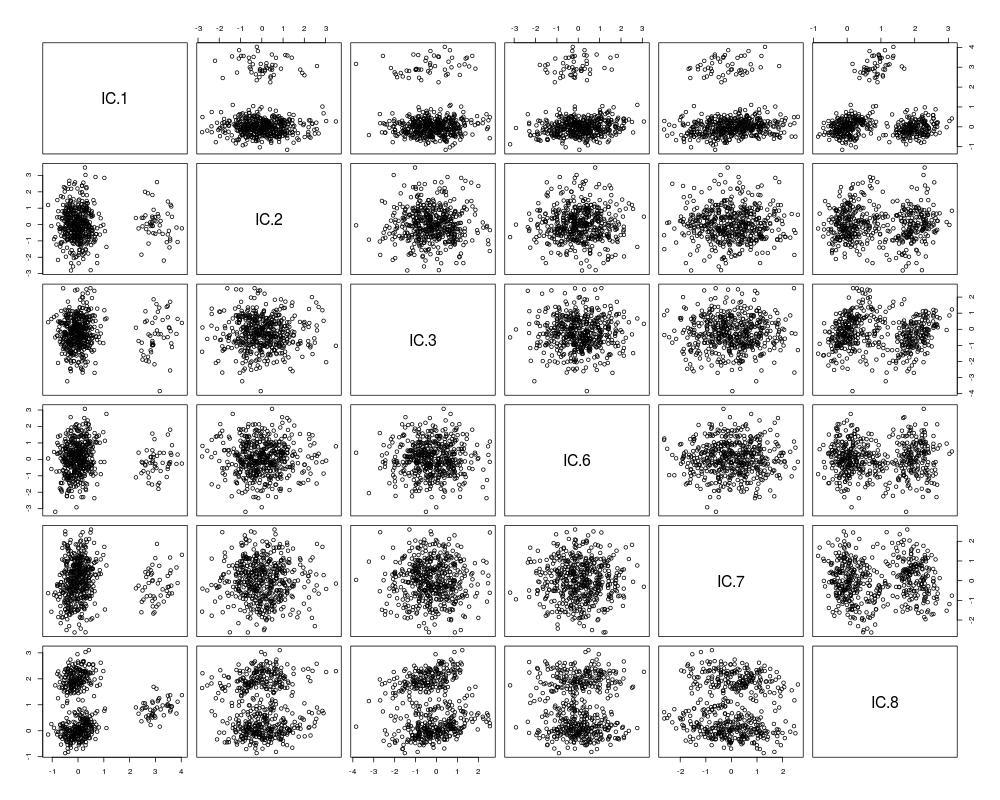
    ics.X.1 <- ics(X)
    summary(ics.X.1)
    plot(ics.X.1)

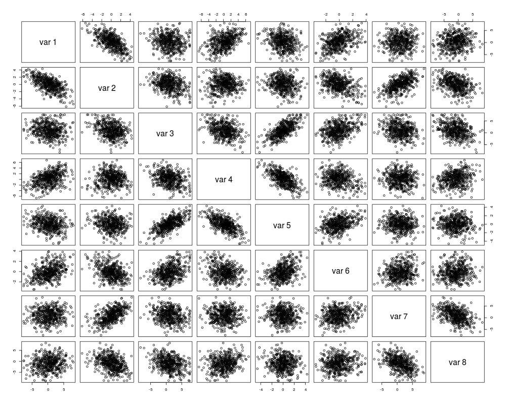
    # compare to
    pairs(X)
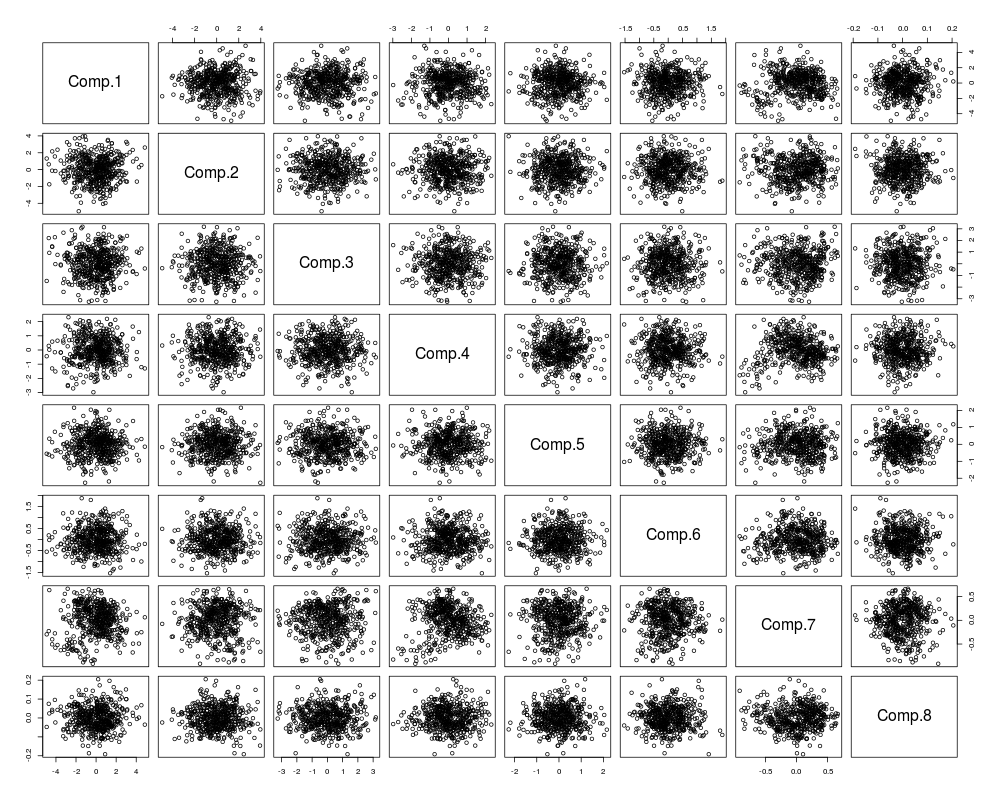
    pairs(princomp(X,cor=TRUE)$scores)

    # slow:
    
    # library(ICSNP)
    # ics.X.2 <- ics(X, tyler.shape, duembgen.shape, S1args=list(location=0))
    # summary(ics.X.2)
    # plot(ics.X.2)
    
    rm(.Random.seed)
    
    # example using two computed scatter matrices for outlier detection
    
    library(robustbase)
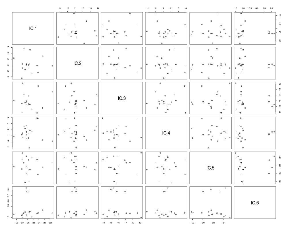
    ics.wood<-ics(wood,tM(wood)$V,tM(wood,2)$V)
    plot(ics.wood)
    
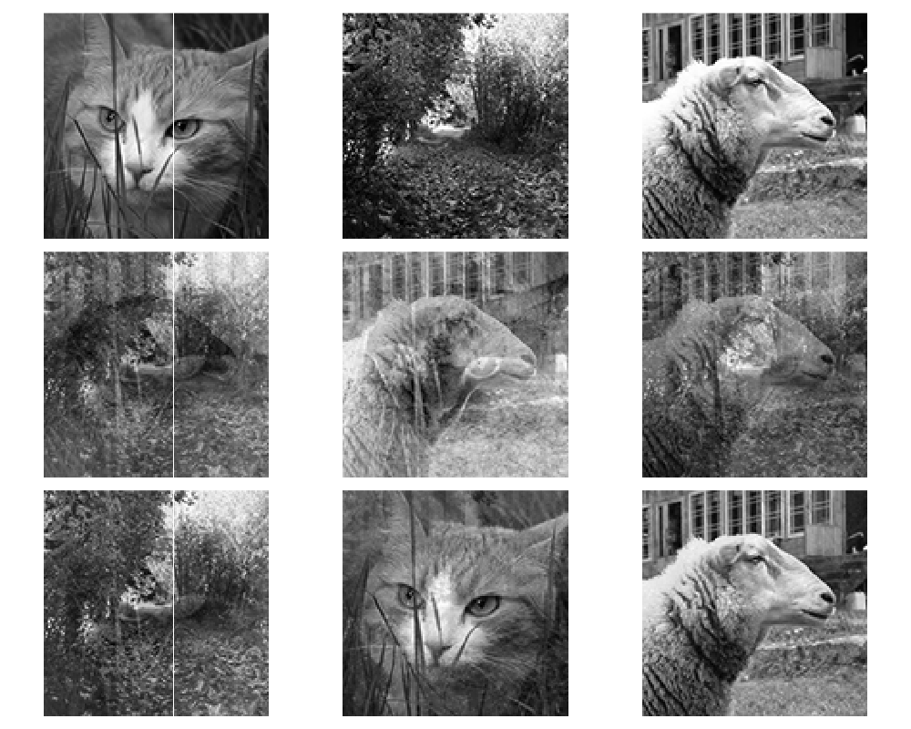
    # example using three pictures
    library(pixmap)
    
    fig1 <- read.pnm(system.file("pictures/cat.pgm", package = "ICS")[1])
    fig2 <- read.pnm(system.file("pictures/road.pgm", package = "ICS")[1])
    fig3 <- read.pnm(system.file("pictures/sheep.pgm", package = "ICS")[1])
    
    p <- dim(fig1@grey)[2]

    fig1.v <- as.vector(fig1@grey)
    fig2.v <- as.vector(fig2@grey)
    fig3.v <- as.vector(fig3@grey)
    X <- cbind(fig1.v,fig2.v,fig3.v)
    
    set.seed(4321)
    A <- matrix(rnorm(9), ncol = 3)
    X.mixed <- X %*% t(A)

    ICA.fig <- ics(X.mixed)
    
    par.old <- par()
    par(mfrow=c(3,3), omi = c(0.1,0.1,0.1,0.1), mai = c(0.1,0.1,0.1,0.1))

    plot(fig1)
    plot(fig2)
    plot(fig3)

    plot(pixmapGrey(X.mixed[,1],ncol=p))
    plot(pixmapGrey(X.mixed[,2],ncol=p))
    plot(pixmapGrey(X.mixed[,3],ncol=p))

    plot(pixmapGrey(ics.components(ICA.fig)[,1],ncol=p))
    plot(pixmapGrey(ics.components(ICA.fig)[,2],ncol=p))
    plot(pixmapGrey(ics.components(ICA.fig)[,3],ncol=p))

    par(par.old)
    rm(.Random.seed)
    

Results

R version 3.3.1 (2016-06-21) -- "Bug in Your Hair"
Copyright (C) 2016 The R Foundation for Statistical Computing
Platform: x86_64-pc-linux-gnu (64-bit)

R is free software and comes with ABSOLUTELY NO WARRANTY.
You are welcome to redistribute it under certain conditions.
Type 'license()' or 'licence()' for distribution details.

R is a collaborative project with many contributors.
Type 'contributors()' for more information and
'citation()' on how to cite R or R packages in publications.

Type 'demo()' for some demos, 'help()' for on-line help, or
'help.start()' for an HTML browser interface to help.
Type 'q()' to quit R.

> library(ICS)
Loading required package: mvtnorm
> png(filename="/home/ddbj/snapshot/RGM3/R_CC/result/ICS/ics.Rd_%03d_medium.png", width=480, height=480)
> ### Name: ics
> ### Title: Two Scatter Matrix ICS Transformation
> ### Aliases: ics
> ### Keywords: models multivariate
> 
> ### ** Examples
> 
>     # example using two functions
>     set.seed(123456)
>     X1 <- rmvnorm(250, rep(0,8), diag(c(rep(1,6),0.04,0.04)))
>     X2 <- rmvnorm(50, c(rep(0,6),2,0), diag(c(rep(1,6),0.04,0.04)))
>     X3 <- rmvnorm(200, c(rep(0,7),2), diag(c(rep(1,6),0.04,0.04)))
> 
>     X.comps <- rbind(X1,X2,X3)
>     A <- matrix(rnorm(64),nrow=8)
>     X <- X.comps %*% t(A)
> 
>     ics.X.1 <- ics(X)
>     summary(ics.X.1)

ICS based on two scatter matrices 
S1:  cov
S2:  cov4

The generalized kurtosis measures of the components are:
[1] 1.2949 1.0808 1.0572 1.0315 0.9904 0.9679 0.9218 0.7415


The Unmixing matrix is:
        [,1]    [,2]    [,3]    [,4]    [,5]    [,6]    [,7]    [,8]
[1,] -0.4048 -1.0060  0.0640 -0.1190 -0.3679 -0.0146  0.5489  0.1722
[2,] -1.9729 -3.6737 -1.2083  1.6144  0.8539  0.6864  0.8519 -0.8023
[3,] -1.1440 -1.3710 -0.7102  0.8597  0.7894  0.8565  0.3838 -0.3897
[4,]  0.8910  1.9038  0.7101 -0.9389 -1.2674 -0.4864 -0.4194  0.6221
[5,]  0.0163 -0.2555 -0.1768  0.2055  0.7280 -0.5341  0.2922  0.1739
[6,] -0.6777 -1.4301 -0.6167  0.2690  0.4775 -0.2117  0.3785 -0.4618
[7,]  1.2681  2.1872  0.5512 -0.8628 -0.8426 -0.0272 -0.4163  0.3730
[8,]  1.0146  1.7801  1.2192 -0.7677 -1.1722 -0.9849  0.0158  0.6356
>     plot(ics.X.1)
> 
>     # compare to
>     pairs(X)
>     pairs(princomp(X,cor=TRUE)$scores)
> 
>     # slow:
>     
>     # library(ICSNP)
>     # ics.X.2 <- ics(X, tyler.shape, duembgen.shape, S1args=list(location=0))
>     # summary(ics.X.2)
>     # plot(ics.X.2)
>     
>     rm(.Random.seed)
>     
>     # example using two computed scatter matrices for outlier detection
>     
>     library(robustbase)
>     ics.wood<-ics(wood,tM(wood)$V,tM(wood,2)$V)
>     plot(ics.wood)
>     
>     # example using three pictures
>     library(pixmap)
>     
>     fig1 <- read.pnm(system.file("pictures/cat.pgm", package = "ICS")[1])
Warning message:
In rep(cellres, length = 2) : 'x' is NULL so the result will be NULL
>     fig2 <- read.pnm(system.file("pictures/road.pgm", package = "ICS")[1])
Warning message:
In rep(cellres, length = 2) : 'x' is NULL so the result will be NULL
>     fig3 <- read.pnm(system.file("pictures/sheep.pgm", package = "ICS")[1])
Warning message:
In rep(cellres, length = 2) : 'x' is NULL so the result will be NULL
>     
>     p <- dim(fig1@grey)[2]
> 
>     fig1.v <- as.vector(fig1@grey)
>     fig2.v <- as.vector(fig2@grey)
>     fig3.v <- as.vector(fig3@grey)
>     X <- cbind(fig1.v,fig2.v,fig3.v)
>     
>     set.seed(4321)
>     A <- matrix(rnorm(9), ncol = 3)
>     X.mixed <- X %*% t(A)
> 
>     ICA.fig <- ics(X.mixed)
>     
>     par.old <- par()
>     par(mfrow=c(3,3), omi = c(0.1,0.1,0.1,0.1), mai = c(0.1,0.1,0.1,0.1))
> 
>     plot(fig1)
>     plot(fig2)
>     plot(fig3)
> 
>     plot(pixmapGrey(X.mixed[,1],ncol=p))
Warning message:
In rep(cellres, length = 2) : 'x' is NULL so the result will be NULL
>     plot(pixmapGrey(X.mixed[,2],ncol=p))
Warning message:
In rep(cellres, length = 2) : 'x' is NULL so the result will be NULL
>     plot(pixmapGrey(X.mixed[,3],ncol=p))
Warning message:
In rep(cellres, length = 2) : 'x' is NULL so the result will be NULL
> 
>     plot(pixmapGrey(ics.components(ICA.fig)[,1],ncol=p))
Warning message:
In rep(cellres, length = 2) : 'x' is NULL so the result will be NULL
>     plot(pixmapGrey(ics.components(ICA.fig)[,2],ncol=p))
Warning message:
In rep(cellres, length = 2) : 'x' is NULL so the result will be NULL
>     plot(pixmapGrey(ics.components(ICA.fig)[,3],ncol=p))
Warning message:
In rep(cellres, length = 2) : 'x' is NULL so the result will be NULL
> 
>     par(par.old)
Warning messages:
1: In par(par.old) : graphical parameter "cin" cannot be set
2: In par(par.old) : graphical parameter "cra" cannot be set
3: In par(par.old) : graphical parameter "csi" cannot be set
4: In par(par.old) : graphical parameter "cxy" cannot be set
5: In par(par.old) : graphical parameter "din" cannot be set
6: In par(par.old) : graphical parameter "page" cannot be set
>     rm(.Random.seed)
>     
> 
> 
> 
> 
> dev.off()
null device 
          1 
>