Supported by Dr. Osamu Ogasawara and  . . |
|
Last data update: 2014.03.03 |
Supervised scatter matrix based on quantilesDescriptionFunction for a supervised scatter matrix that is the weighted
covariance matrix of Usage
scovq(x, y, q1 = 0, q2 = 0.5, pos = TRUE, type = 7,
      method = "unbiased", na.action = na.fail,
      check = TRUE)
Arguments
DetailsThe weights for this supervised scatter matrix for scovq = ∑ w(y) (x-x_w_bar)'(x-x_w_bar). where x_w_bar = sum w(y)x. To see how this function can be used in the context of supervised invariant coordinate selection see the example below. Valuea matrix. Author(s)Klaus Nordhausen ReferencesLiski, E., Nordhausen, K. and Oja, H. (2013), Supervised invariant coordinate selection, To appear in Statistics, ???, ???–???. See Also
Examples
# Creating some data
# The number of explaining variables
p <- 10
# The number of observations
n <- 400
# The error variance
sigma <- 0.5
# The explaining variables
X <- matrix(rnorm(p*n),n,p)
# The error term
epsilon <- rnorm(n, sd = sigma)
# The response
y <- X[,1]^2 + X[,2]^2*epsilon
# SICS with ics
X.centered <- sweep(X,2,colMeans(X),"-")
SICS <- ics(X.centered, S1=cov, S2=scovq, S2args=list(y=y, q1=0.25,
q2=0.75, pos=FALSE), stdKurt=FALSE, stdB="Z")
# Assuming it is known that k=2, then the two directions
# of interest are choosen as:
k <- 2
KURTS <- SICS@gKurt
KURTS.max <- ifelse(KURTS >= 1, KURTS, 1/KURTS)
ordKM <- order(KURTS.max, decreasing = TRUE)
indKM <- ordKM[1:k]
# The two variables of interest
Zk <- ics.components(SICS)[,indKM]
# The correspondings transformation matrix
Bk <- coef(SICS)[indKM,]
# The corresponding projection matrix
Pk <- t(Bk) %*% solve(Bk %*% t(Bk)) %*% Bk
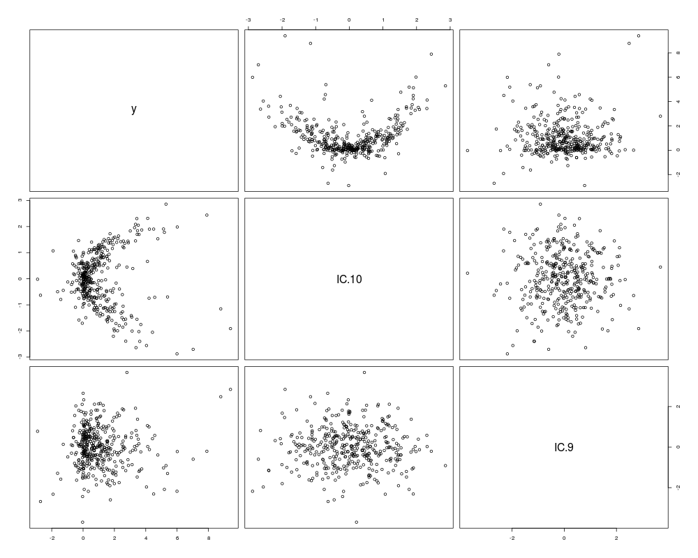
# Visualization
pairs(cbind(y,Zk))
# checking the subspace difference
# true projection
B0 <- rbind(rep(c(1,0),c(1,p-1)),rep(c(0,1,0),c(1,1,p-2)))
P0 <- t(B0) %*% solve(B0 %*% t(B0)) %*% B0
# crone and crosby subspace distance measure, should be small
k - sum(diag(P0 %*% Pk))
Results
R version 3.3.1 (2016-06-21) -- "Bug in Your Hair"
Copyright (C) 2016 The R Foundation for Statistical Computing
Platform: x86_64-pc-linux-gnu (64-bit)

R is free software and comes with ABSOLUTELY NO WARRANTY.
You are welcome to redistribute it under certain conditions.
Type 'license()' or 'licence()' for distribution details.

R is a collaborative project with many contributors.
Type 'contributors()' for more information and
'citation()' on how to cite R or R packages in publications.

Type 'demo()' for some demos, 'help()' for on-line help, or
'help.start()' for an HTML browser interface to help.
Type 'q()' to quit R.

> library(ICS)
Loading required package: mvtnorm
> png(filename="/home/ddbj/snapshot/RGM3/R_CC/result/ICS/scovq.Rd_%03d_medium.png", width=480, height=480)
> ### Name: scovq
> ### Title: Supervised scatter matrix based on quantiles
> ### Aliases: scovq
> ### Keywords: multivariate
>
> ### ** Examples
>
> # Creating some data
>
> # The number of explaining variables
> p <- 10
> # The number of observations
> n <- 400
> # The error variance
> sigma <- 0.5
> # The explaining variables
> X <- matrix(rnorm(p*n),n,p)
> # The error term
> epsilon <- rnorm(n, sd = sigma)
> # The response
> y <- X[,1]^2 + X[,2]^2*epsilon
>
>
> # SICS with ics
>
> X.centered <- sweep(X,2,colMeans(X),"-")
> SICS <- ics(X.centered, S1=cov, S2=scovq, S2args=list(y=y, q1=0.25,
+         q2=0.75, pos=FALSE), stdKurt=FALSE, stdB="Z")
>
> # Assuming it is known that k=2, then the two directions
> # of interest are choosen as:
>
> k <- 2
> KURTS <- SICS@gKurt
> KURTS.max <- ifelse(KURTS >= 1, KURTS, 1/KURTS)
> ordKM <- order(KURTS.max, decreasing = TRUE)
>
> indKM <- ordKM[1:k]
>
> # The two variables of interest
> Zk <- ics.components(SICS)[,indKM]
>
> # The correspondings transformation matrix
> Bk <- coef(SICS)[indKM,]
>
> # The corresponding projection matrix
> Pk <- t(Bk) %*% solve(Bk %*% t(Bk)) %*% Bk
>
> # Visualization
> pairs(cbind(y,Zk))
>
> # checking the subspace difference
>
> # true projection
>
> B0 <- rbind(rep(c(1,0),c(1,p-1)),rep(c(0,1,0),c(1,1,p-2)))
> P0 <- t(B0) %*% solve(B0 %*% t(B0)) %*% B0
>
> # crone and crosby subspace distance measure, should be small
> k - sum(diag(P0 %*% Pk))
[1] 0.5934633
>
>
>
>
>
>
> dev.off()
null device
          1
>
|