R Graphical Manual

Browse All

Last data update: 2014.03.03

R: Image Lag Plot Matrix for Large Time Series

ilagplot

R Documentation

Image Lag Plot Matrix for Large Time Series

Description

Produces an image lag plot matrix of large timeseries where the colors encode the density of the points in the lag plots.

Usage

ilagplot(x, set.lags = 1,
         pixs = 1, zmax = NULL, ztransf = function(x){x},
         colramp = IDPcolorRamp, mfrow=NULL, cex=par("cex"),
         main = NULL, d.main = 1, cex.main = 1.5*par("cex.main"),
         legend = TRUE, d.legend = 1,
         cex.axis = par("cex.axis"), las = 1,
         border=FALSE, mar = c(2,2,2,0), oma = rep(0,4)+0.1,
         mgp = c(2,0.5,0)*cex.axis, tcl = -0.3, ...)

Arguments

`x`	ts object or ordinary vector
`set.lags`	vector of lags to be displayed
`pixs`	Pixel size in mm
`zmax`	Maximum counts per Pixel to be plotted. When NULL each lag plot has its individual scale. If a number >= maximum number of counts per pixel is supplied, the scale will be identical for all lag plots. The maximum of the number per pixel is delivered by the return value. Beware: `zmax` has its meaning only for ilagplots with identical settings for main, legend, mar and oma!
`ztransf`	Function to transform the counts. The user has to make sure that the transformed counts lie in the range [0,zmax], where zmax is any positive number (>=2).
`colramp`	Color ramp to encode the density of the points within a pixel
`mfrow`	See Argument `mfrow` in `par`
`cex`	See Argument `cex` in `par`
`main`	Title
`d.main`	Vertical distance between upper border of scatter plots and the title line in multiples of title height.
`cex.main`	Magnification used for title relative to the current setting of cex.
`legend`	Logical. When `FALSE`, no legend is plotted and space is saved in figure region.
`d.legend`	Horizontal distance between right border of scatter plots and legend in multiples of title height.
`cex.axis`	Magnification used for axis annotation relative to the current setting of cex.
`las`	Orientation of labels on axes.
`border`	Logical. When `TRUE`, a border is drawn around the individual colors in the legend.
`mar, oma`	Margin and outer margin respectively. Cf. `par`
`mgp, tcl`	Cf. `par`
`...`	Additional arguments to `par`

Details

Code is based on R function lag.plot V1.7. Tip: Legend looks better when mar is defined symmetrically.

Value

Maximum number of counts per Pixel found.

Note

When you get the error message "Zmax too small! Densiest aereas are out of range!" you must run the function with identical parameters but without specifying zmax. The value returned gives you the minimum value allowed for zmax.

Author(s)

Andreas Ruckstuhl, refined by Rene Locher

Examples

if(require(SwissAir)) {
  data(AirQual)

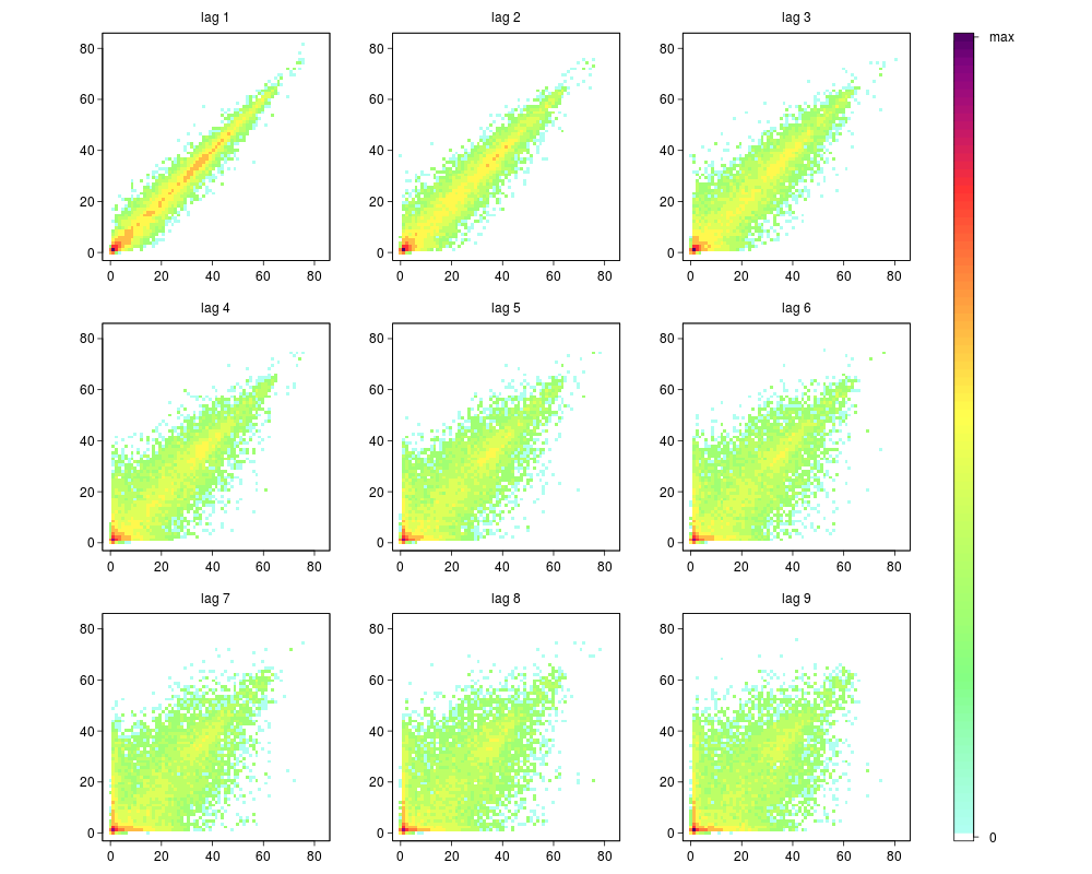
  ## low correlation
  ilagplot(AirQual[,c("ad.O3")],set.lags = 1:9,
         ztransf=function(x){x[x<1] <- 1; log2(x)})

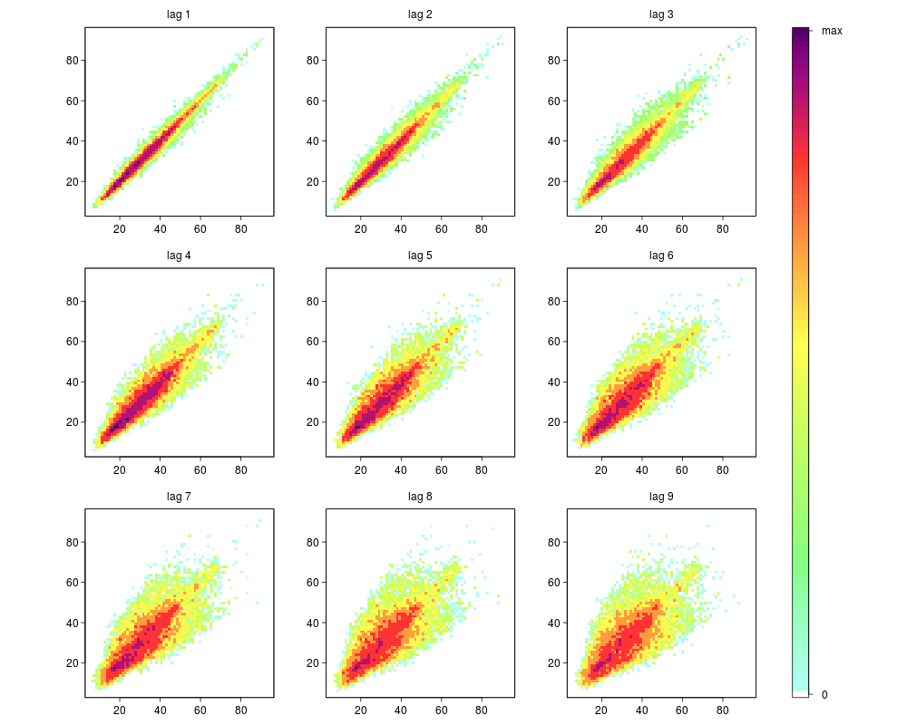
  ## high correlation
  Ox <- AirQual[,c("ad.O3","lu.O3","sz.O3")]+
    AirQual[,c("ad.NOx","lu.NOx","sz.NOx")]-
      AirQual[,c("ad.NO","lu.NO","sz.NO")]
  names(Ox) <- c("ad","lu","sz")
  ilagplot(Ox$ad,set.lags = 1:9,
           ztransf=function(x){x[x<1] <- 1; log2(x)})

  ## cf. ?AirQual for the explanation of the physical
  ## and chemical background
} else print("Package SwissAir is not available")

Results


R version 3.3.1 (2016-06-21) -- "Bug in Your Hair"
Copyright (C) 2016 The R Foundation for Statistical Computing
Platform: x86_64-pc-linux-gnu (64-bit)

R is free software and comes with ABSOLUTELY NO WARRANTY.
You are welcome to redistribute it under certain conditions.
Type 'license()' or 'licence()' for distribution details.

R is a collaborative project with many contributors.
Type 'contributors()' for more information and
'citation()' on how to cite R or R packages in publications.

Type 'demo()' for some demos, 'help()' for on-line help, or
'help.start()' for an HTML browser interface to help.
Type 'q()' to quit R.

> library(IDPmisc)
Loading required package: grid
Loading required package: lattice
> png(filename="/home/ddbj/snapshot/RGM3/R_CC/result/IDPmisc/ilagplot.Rd_%03d_medium.png", width=480, height=480)
> ### Name: ilagplot
> ### Title: Image Lag Plot Matrix for Large Time Series
> ### Aliases: ilagplot
> ### Keywords: hplot
> 
> ### ** Examples
> 
> if(require(SwissAir)) {
+   data(AirQual)
+ 
+   ## low correlation
+   ilagplot(AirQual[,c("ad.O3")],set.lags = 1:9,
+          ztransf=function(x){x[x<1] <- 1; log2(x)})
+ 
+   ## high correlation
+   Ox <- AirQual[,c("ad.O3","lu.O3","sz.O3")]+
+     AirQual[,c("ad.NOx","lu.NOx","sz.NOx")]-
+       AirQual[,c("ad.NO","lu.NO","sz.NO")]
+   names(Ox) <- c("ad","lu","sz")
+   ilagplot(Ox$ad,set.lags = 1:9,
+            ztransf=function(x){x[x<1] <- 1; log2(x)})
+ 
+   ## cf. ?AirQual for the explanation of the physical
+   ## and chemical background
+ } else print("Package SwissAir is not available")
Loading required package: SwissAir
> 
> 
> 
> 
> 
> dev.off()
null device 
          1 
>