R Graphical Manual

Browse All

Last data update: 2014.03.03

R: Image Scatter Plot for Large Datasets

iplot

R Documentation

Image Scatter Plot for Large Datasets

Description

Produces an image scatter plot of large datasets where the colors encode the density of the points in the scatter plot. Works also with factors.

Usage

iplot(x, y = NULL,
      pixs = 1, zmax = NULL, ztransf = function(x){x},
      colramp = IDPcolorRamp, cex = par("cex"),
      main = NULL, d.main = 1, cex.main = par("cex.main"),
      xlab = NULL, ylab = NULL, cex.lab = 1,
      legend = TRUE, d.legend = 1,
      cex.axis = par("cex.axis"), nlab.xaxis = 5, nlab.yaxis = 5,
      minL.axis = 3, las = 1, border = FALSE,
      oma = c(5,4,1,0)+0.1, mgp = c(2,0.5,0)*cex.axis, tcl = -0.3, ...
      )

Arguments

`x,y`	Coordinates of points whose density is to be plotted. If `x` ist a matrix or a data.frame, the first two column are used as x and y respectively. `y` must be in this case NULL. `x` and `y` may be numeric or factor variable.
`pixs`	Pixelsize in mm.
`zmax`	Maximum number of counts per pixel in the plot. When `NULL`, the density in the scatter plot is encoded from 0 to maximum number of counts per pixel observed. `zmax` must be equal or larger than maximum number of counts found. The maximum number of counts per pixel is delivered by the return value.
`ztransf`	Function to transform the number of counts per pixel, which will be mapped by the function in `colramp` to well defined colors. The user has to make sure that the transformed density lies in the range [0,zmax], where zmax is any positive number (>=2). For examples see `ipairs` and `ilagplot`.
`colramp`	Color ramp to encode the number of counts within a pixel.
`cex`	Magnification of text relative to default.
`main`	Title.
`d.main`	Vertical distance between upper border of scatter plots and the title line in multiples of title height.
`cex.main`	Magnification used for title relative to the current setting of cex.
`xlab`	Label for x-axis.
`ylab`	Label for y-axis.
`cex.lab`	Magnification used for text in axis labels relative to the current setting of cex
`legend`	Logical. When `FALSE`, no legend is plotted and space is saved in figure region.
`d.legend`	Horizontal distance between right border of scatter plot and legend in multiples of title height.
`cex.axis`	Magnification used for axis annotation relative to the current setting of cex.
`nlab.xaxis, nlab.yaxis`	Approximate number of labels on x- and y-axes respectively.
`minL.axis`	The minimum length of the abbreviations of factor levels, used to label the axes ticks.
`las`	Orientation of labels on axes.
`border`	Logical. When `TRUE`, a border is drawn around the individual colors in the legend.
`oma`	Outer margin. Cf. `par`
`mgp, tcl`	Cf. `par`
`...`	Additional arguments to `par`

Details

The idea of this plot is similar to gplot.hexbin. The hexagons are better suited to reflect the density of points in a plane than the squares used here. Nevertheless squares are, contrary to hexagons, invariant to reflexions at the x- and y-axis and therefore suited for scatter plot matrices and also for plotting factors.

Value

Maximum number of counts per Pixel found.

Note

When you get the error message "Zmax too small! Densiest aereas are out of range!" you must run the function again without specifying zmax. The value returned gives you the minimum value allowed for zmax.

Author(s)

Andreas Ruckstuhl, Rene Locher

Examples

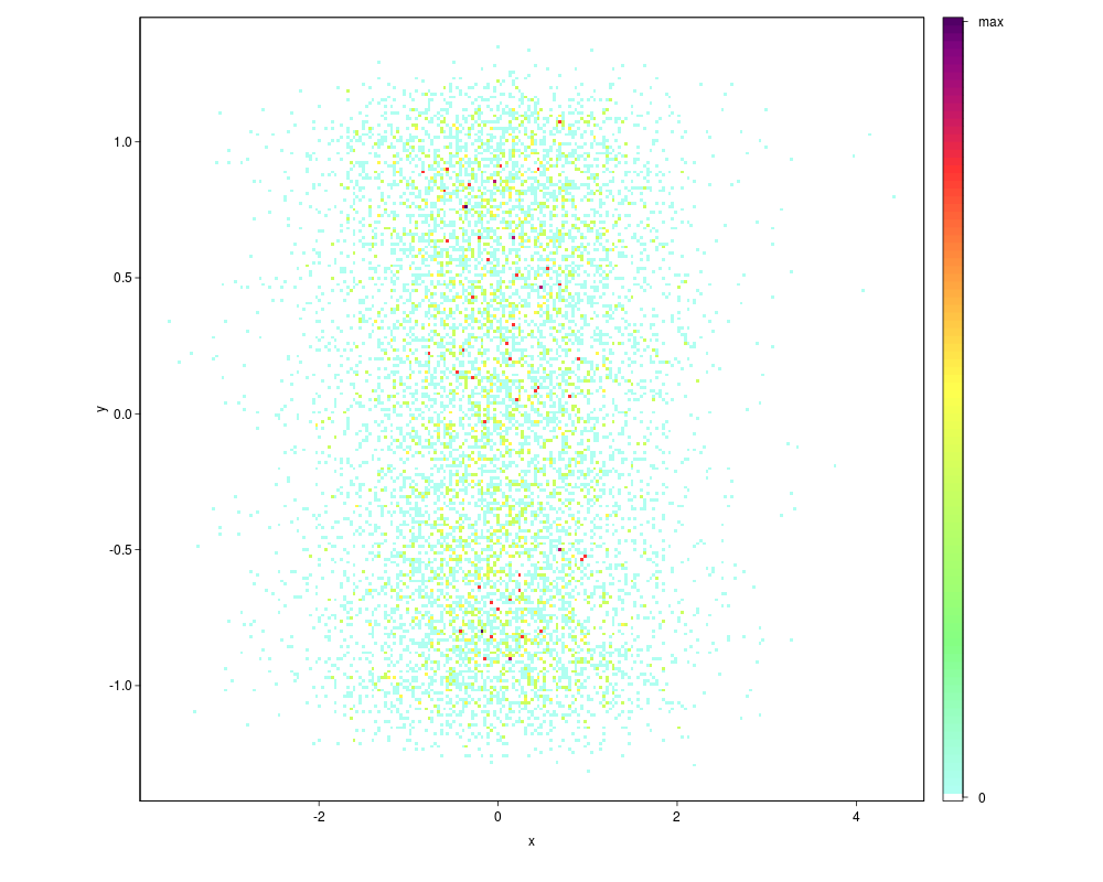
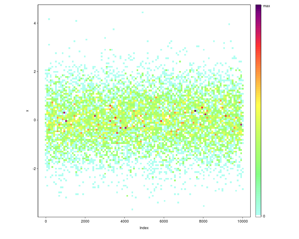
x <-  rnorm(10000)
y <- atan(rnorm(10000, 0))
iplot(x, y)
iplot(x, pixs=2)

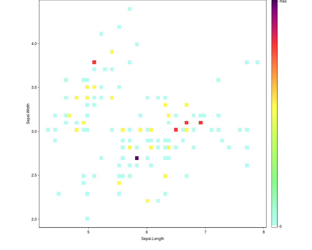
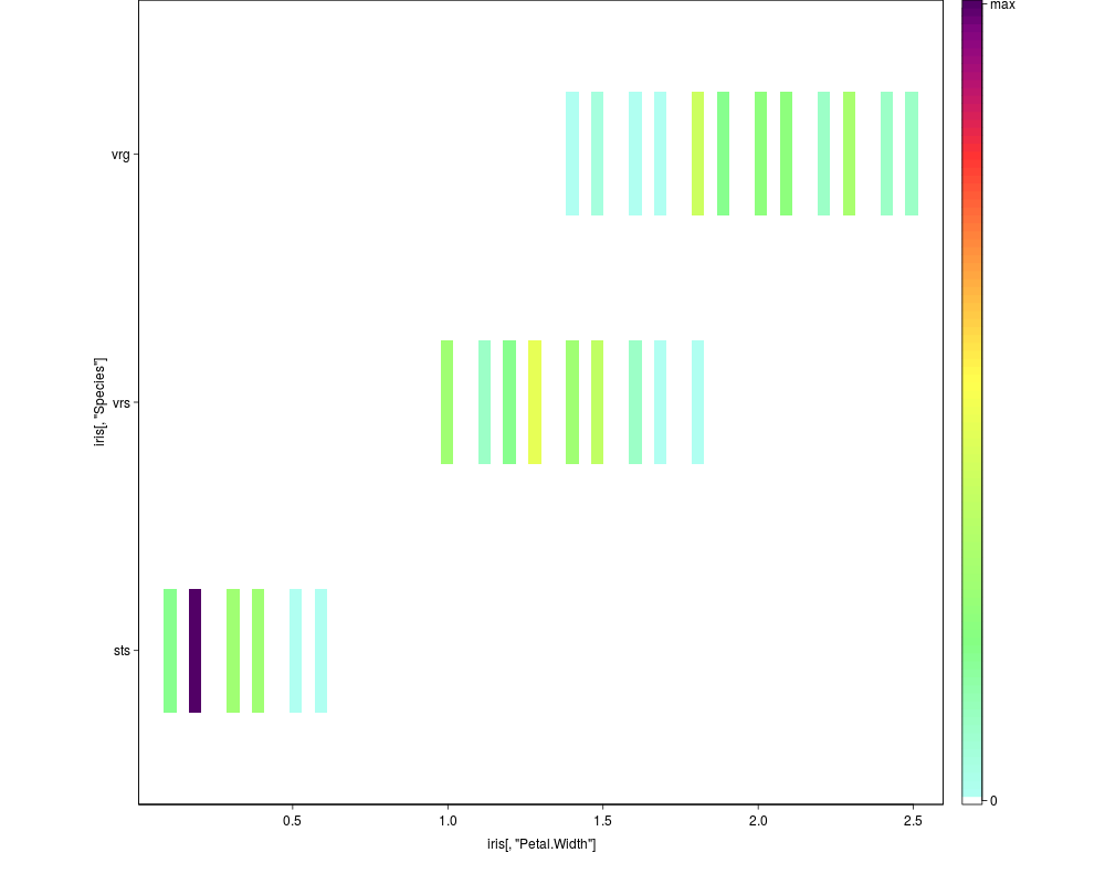
oma <- c(5,5,0,0)
iplot(iris[,1:2],pixs=4, oma=oma)
iplot(iris[,"Petal.Width"], iris[,"Species"], pixs=4, oma=oma)
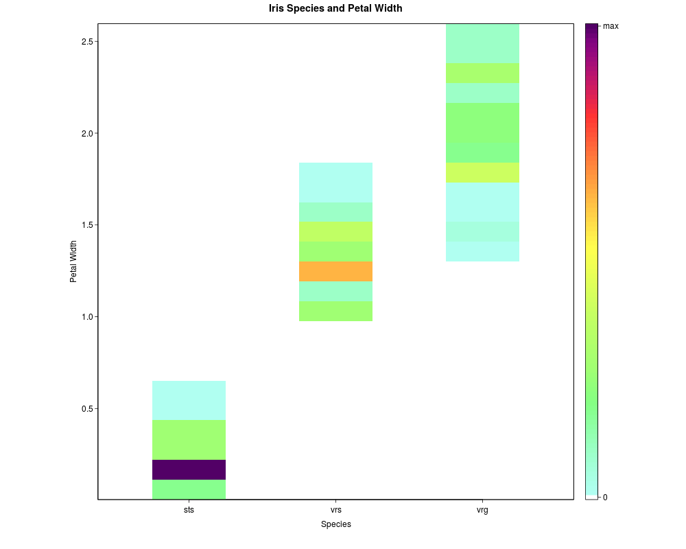
iplot(x=iris[,"Species"], y=iris[,"Petal.Width"], pixs=10,border=TRUE,
        xlab="Species",
        ylab="Petal Width",
        main="Iris Species and Petal Width", oma=oma)

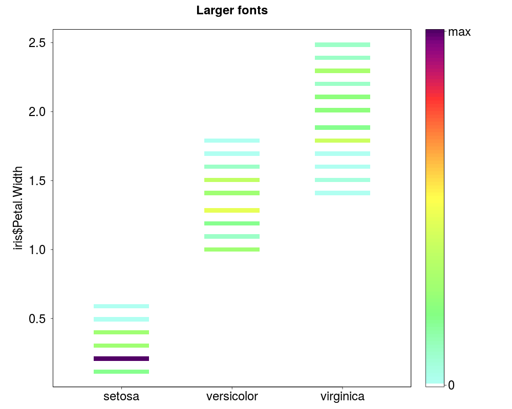
iplot(iris$Species, iris$Petal.Width,pixs=3, minL.axis=10,
      oma=c(3,6,0,0), mgp=c(4, 1, 0),
      cex.axis=2, cex.lab=2, cex.main= 2, main="Larger fonts")

Results


R version 3.3.1 (2016-06-21) -- "Bug in Your Hair"
Copyright (C) 2016 The R Foundation for Statistical Computing
Platform: x86_64-pc-linux-gnu (64-bit)

R is free software and comes with ABSOLUTELY NO WARRANTY.
You are welcome to redistribute it under certain conditions.
Type 'license()' or 'licence()' for distribution details.

R is a collaborative project with many contributors.
Type 'contributors()' for more information and
'citation()' on how to cite R or R packages in publications.

Type 'demo()' for some demos, 'help()' for on-line help, or
'help.start()' for an HTML browser interface to help.
Type 'q()' to quit R.

> library(IDPmisc)
Loading required package: grid
Loading required package: lattice
> png(filename="/home/ddbj/snapshot/RGM3/R_CC/result/IDPmisc/iplot.Rd_%03d_medium.png", width=480, height=480)
> ### Name: iplot
> ### Title: Image Scatter Plot for Large Datasets
> ### Aliases: iplot
> ### Keywords: hplot
> 
> ### ** Examples
> 
> x <-  rnorm(10000)
> y <- atan(rnorm(10000, 0))
> iplot(x, y)
> iplot(x, pixs=2)
> 
> oma <- c(5,5,0,0)
> iplot(iris[,1:2],pixs=4, oma=oma)
> iplot(iris[,"Petal.Width"], iris[,"Species"], pixs=4, oma=oma)
> iplot(x=iris[,"Species"], y=iris[,"Petal.Width"], pixs=10,border=TRUE,
+         xlab="Species",
+         ylab="Petal Width",
+         main="Iris Species and Petal Width", oma=oma)
> 
> iplot(iris$Species, iris$Petal.Width,pixs=3, minL.axis=10,
+       oma=c(3,6,0,0), mgp=c(4, 1, 0),
+       cex.axis=2, cex.lab=2, cex.main= 2, main="Larger fonts")
> 
> 
> 
> 
> 
> dev.off()
null device 
          1 
>