Supported by Dr. Osamu Ogasawara and  . . |
|
Last data update: 2014.03.03 |
Plot Very Long Regular Time SeriesDescriptionPlot one or more regular time series in multiple figures on one or more pages. Usage
longtsPlot(y1, y2 = NULL,
           names1 = NULL, names2 = NULL,
           startP = start(y1)[1], upf = 400, fpp = 4, overlap = 20,
           x.at = NULL, x.ann = NULL, x.tick = NULL,
           y1.at = NULL, y1.ann = NULL, y1.tick = NULL,
           y2.at = NULL, y2.ann = NULL, y2.tick = NULL,
           nx.ann = 10, ny.ann = 3, cex.ann = par("cex.axis"),
           xlab = "", y1lab = "", y2lab = "", las = 0,
           col.y1 = "black", col.y2 = col.y1,
           cex.lab = par("cex.lab"),
           y1lim = range(y1, na.rm = TRUE, finite=TRUE),
           y2lim = range(y2, na.rm = TRUE, finite=TRUE),
           lty1 = 1, lty2 = 2, lwd1 = 1, lwd2 = lwd1,
           col1 = NULL, col2 = NULL,
           leg = TRUE, y1nam.leg = NULL, y2nam.leg = NULL,
           ncol.leg = NULL, cex.leg = par("cex"),
           h1 = NULL, h2 = NULL, col.h1 = "gray70", col.h2 = "gray70",
           main = NULL, cex.main = par("cex.main"),
           automain = is.null(main),
           mgp = c(2, 0.7, 0), mar = c(2,3,1,3)+.2,
           oma = if (automain|!is.null(main))
                             c(0,0,2,0) else par("oma"),
           xpd = par("xpd"), cex = par("cex"),
           type1 = "s", type2 = type1,
           pch1 = 46, pch2 = pch1, cex.pt1 = 2, cex.pt2 = cex.pt1,
           slide = FALSE, each.fig = 1,
           filename = NULL, extension = NULL, filetype = NULL, ...)
Arguments
DetailsFor longer time-series, it is sometimes important to spread several
time-series plots over several subplots or even over several pages
with several subplots in each. Moreover, these series have often
different ranges, frequencies and start times. There is sometimes also
the need of a more flexible annotation of axes than Side EffectsOne or more pages of time series plots are drawn on the current graphic device and, optionally, saved in one or more files. Author(s)Rene Locher Examples
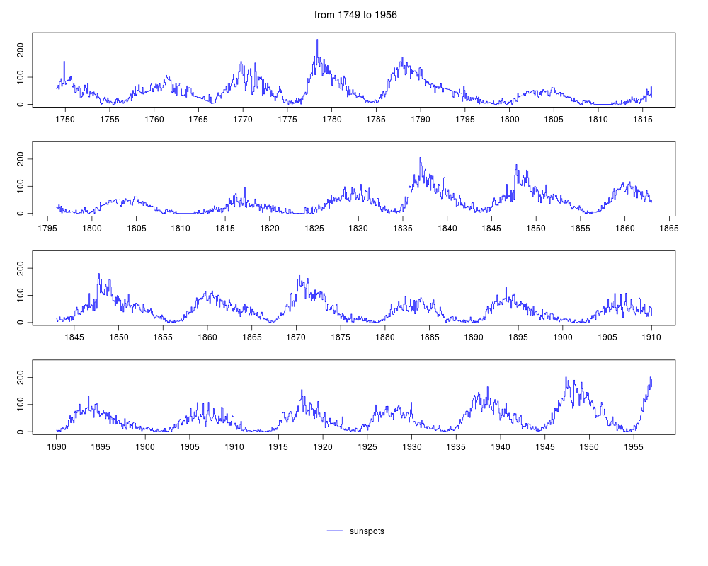
## sunspots, y-axis only on the left
data(sunspots)
longtsPlot(sunspots,upf=ceiling((end(sunspots)-start(sunspots))[1]/5))
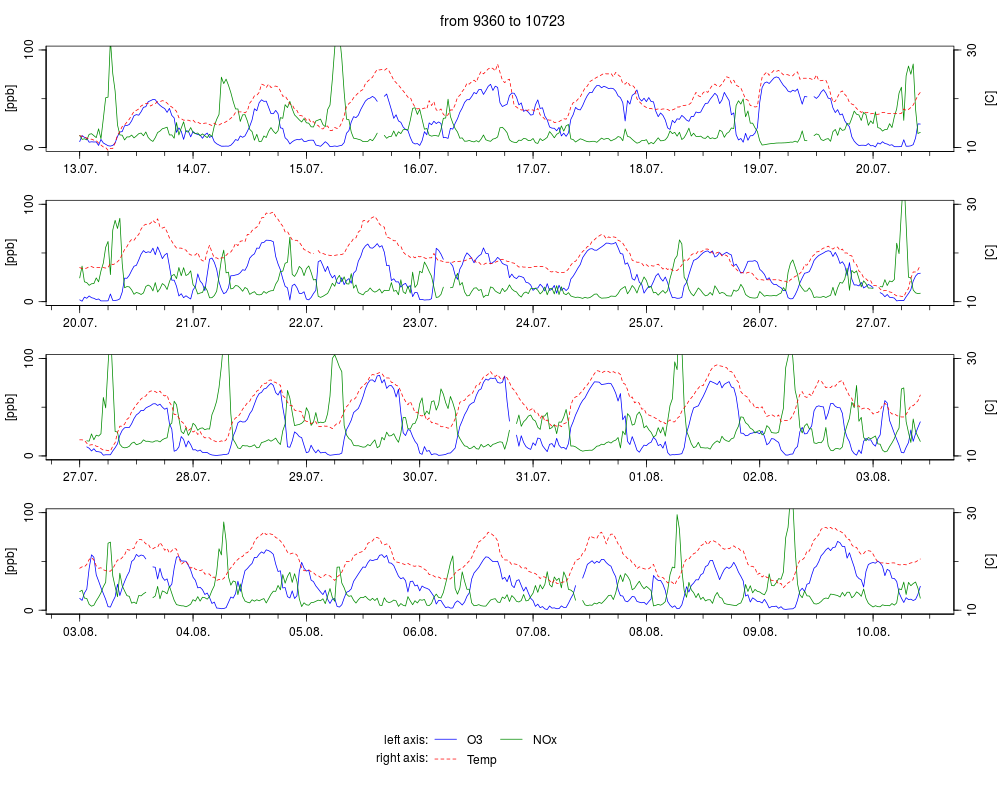
## air quality (left axis) and meteo data (right axis)
## use xpd=TRUE for time series with rare but large values
if (require(SwissAir)) {
data(AirQual)
st <- 6.5*30*48
x.at <- seq(st,nrow(AirQual),48)
longtsPlot(y1=AirQual[,c("ad.O3","ad.NOx")], y2 = AirQual$ad.T,
names1=c("O3","NOx"),names2 = "Temp",
startP = st, upf=7*48,
x.at = x.at, x.ann = substr(AirQual$start,1,6)[x.at],
x.tick = seq(st,nrow(AirQual),12),
y1.at = c(0,100), y1.tick = seq(0,150,50),
y2.at = c(10,30), y2.tick = seq(10,30,10),
y1lab="[ppb]", y2lab="[C]",
y1lim = c(0,100), y2lim = c(10,30), xpd=TRUE,
col2 = "red", type1 = "l")
}
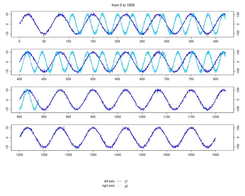
## Two time series with different frequencies and start times
## on the same figures
set.seed(13)
len <- 4*6*400
x <- sin((1:len)/200*pi)
d <- sin(cumsum(1+ rpois(len, lambda= 2.5)))
y1 <- ts(10*x,start=0,frequency=6)+d*rnorm(len)
y2 <- ts(100*x,start=100,frequency=13)+10*rnorm(len)
longtsPlot(y1,y2)
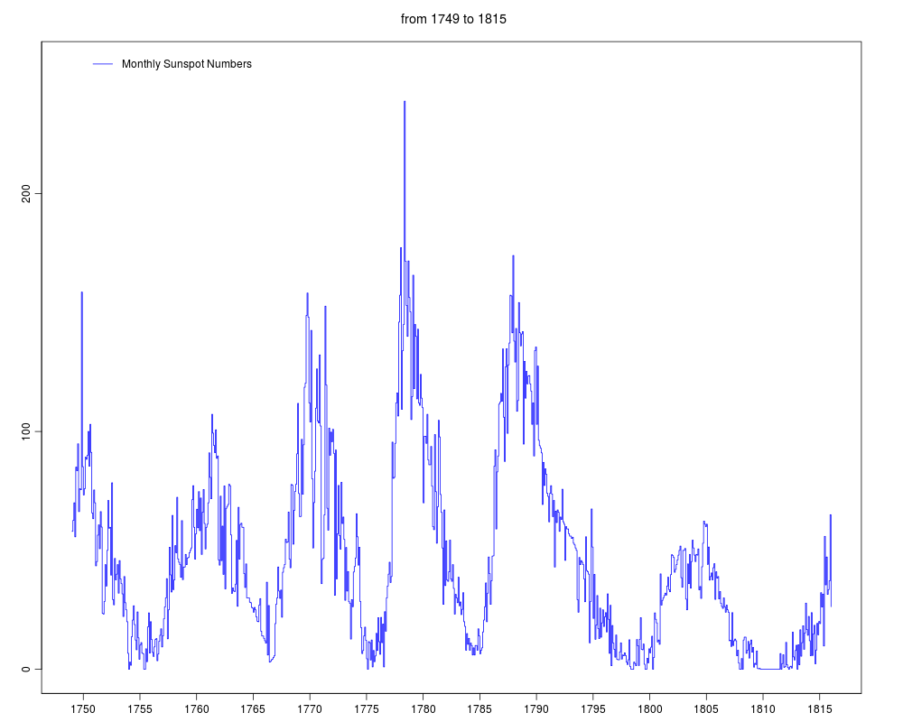
## plot your own legend
longtsPlot(sunspots,upf=ceiling((end(sunspots)-start(sunspots))[1]/5),
fpp=1, leg=FALSE)
legend(1750,260,legend="Monthly Sunspot Numbers",col="blue",lwd=1,
bty="n")
Results
R version 3.3.1 (2016-06-21) -- "Bug in Your Hair"
Copyright (C) 2016 The R Foundation for Statistical Computing
Platform: x86_64-pc-linux-gnu (64-bit)

R is free software and comes with ABSOLUTELY NO WARRANTY.
You are welcome to redistribute it under certain conditions.
Type 'license()' or 'licence()' for distribution details.

R is a collaborative project with many contributors.
Type 'contributors()' for more information and
'citation()' on how to cite R or R packages in publications.

Type 'demo()' for some demos, 'help()' for on-line help, or
'help.start()' for an HTML browser interface to help.
Type 'q()' to quit R.

> library(IDPmisc)
Loading required package: grid
Loading required package: lattice
> png(filename="/home/ddbj/snapshot/RGM3/R_CC/result/IDPmisc/longtsPlot.Rd_%03d_medium.png", width=480, height=480)
> ### Name: longtsPlot
> ### Title: Plot Very Long Regular Time Series
> ### Aliases: longtsPlot
> ### Keywords: hplot iplot ts multivariate
>
> ### ** Examples
>
> ## sunspots, y-axis only on the left
> data(sunspots)
> longtsPlot(sunspots,upf=ceiling((end(sunspots)-start(sunspots))[1]/5))
>
> ## air quality (left axis) and meteo data (right axis)
> ## use xpd=TRUE for time series with rare but large values
> if (require(SwissAir)) {
+   data(AirQual)
+   st <- 6.5*30*48
+   x.at <- seq(st,nrow(AirQual),48)
+   longtsPlot(y1=AirQual[,c("ad.O3","ad.NOx")], y2 = AirQual$ad.T,
+              names1=c("O3","NOx"),names2 = "Temp",
+              startP = st, upf=7*48,
+              x.at = x.at, x.ann = substr(AirQual$start,1,6)[x.at],
+              x.tick = seq(st,nrow(AirQual),12),
+              y1.at = c(0,100), y1.tick = seq(0,150,50),
+              y2.at = c(10,30), y2.tick = seq(10,30,10),
+              y1lab="[ppb]", y2lab="[C]",
+              y1lim = c(0,100), y2lim = c(10,30), xpd=TRUE,
+              col2 = "red", type1 = "l")
+ }
Loading required package: SwissAir
>
> ## Two time series with different frequencies and start times
> ## on the same figures
> set.seed(13)
> len <- 4*6*400
> x <- sin((1:len)/200*pi)
> d <- sin(cumsum(1+ rpois(len, lambda= 2.5)))
>
> y1 <- ts(10*x,start=0,frequency=6)+d*rnorm(len)
> y2 <- ts(100*x,start=100,frequency=13)+10*rnorm(len)
> longtsPlot(y1,y2)
>
> ## plot your own legend
> longtsPlot(sunspots,upf=ceiling((end(sunspots)-start(sunspots))[1]/5),
+            fpp=1, leg=FALSE)
> legend(1750,260,legend="Monthly Sunspot Numbers",col="blue",lwd=1,
+        bty="n")
>
>
>
>
>
> dev.off()
null device
          1
>
|