Supported by Dr. Osamu Ogasawara and  . . |
|
Last data update: 2014.03.03 |
Robust Fitting of BaselinesDescriptionRobust fitting of local regression models for estimating a baseline or a background signal Usage
rfbaseline(x, y, span = 2/3, NoXP = NULL,
           maxit = c(2, 2), b = 3.5, weight = NULL,
           Scale = function(r) median(abs(r))/0.6745,
           delta = NULL, SORT = TRUE, DOT = FALSE, init = NULL)
Arguments
ValueList containing components
Author(s)Andreas Ruckstuhl ReferencesRuckstuhl, Andreas F., Matthew P. Jacobson, Robert W. Field and James A. Dodd (2001); Baseline Subtraction Using Robust Local Regression Estimation; Journal of Quantitative Spectroscopy and Radiative Transfer 68: 179 – 193 Ruckstuhl, Andreas F., et al.; Estimation of background concentrations of atmospheric trace gases using robust local regression; to be published See Also See Also as Examples
data(MS)
MS1 <- log10(MS[MS$mz>12000&MS$mz<1e5,])
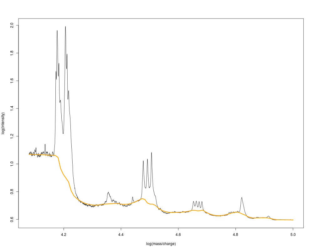
MS1.rfb2 <- rfbaseline(x=MS1$mz, y=MS1$I, NoXP=2200, maxit=c(5,0))
plot(x=MS1$mz, y=MS1$I, type="l",
xlab="log(mass/charge)", ylab="log(intensity)")
lines(MS1.rfb2$x, MS1.rfb2$fit, col="orange", lwd=3)
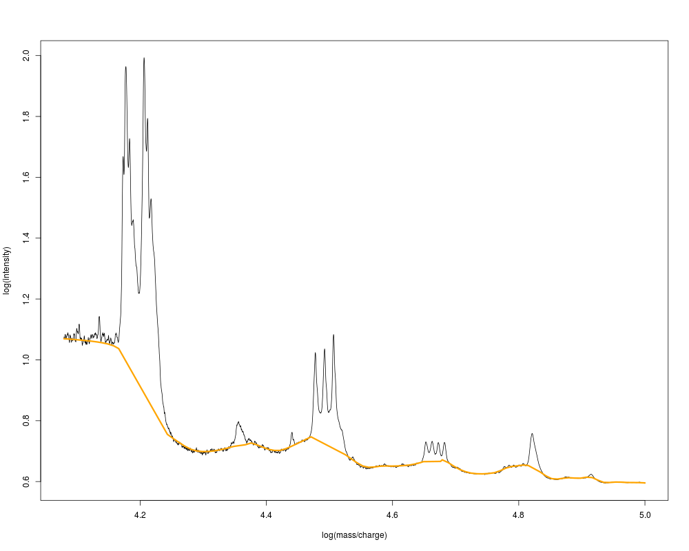
MS1.rfb3 <- rfbaseline(x=MS1$mz, y=MS1$I, NoXP=1100, maxit=c(5,0),
DOT=TRUE, Scale=function(x) mad(x, center=0))
plot(x=MS1$mz, y=MS1$I, type="l",
xlab="log(mass/charge)", ylab="log(intensity)")
lines(MS1.rfb3$x, MS1.rfb3$fit, col="orange", lwd=3)
## 'delta=0' needs much more computer time
## Not run:
MS1.rfb4 <- rfbaseline(x=MS1$mz, y=MS1$I, NoXP=2200,
delta=0, maxit=c(5,0))
plot(x=MS1$mz, y=MS1$I,ty="l",
xlab="log(mass/charge)", ylab="log(intensity)")
lines(MS1.rfb4$x, MS1.rfb4$fit, col="orange", lwd=3)
## End(Not run)
Results
R version 3.3.1 (2016-06-21) -- "Bug in Your Hair"
Copyright (C) 2016 The R Foundation for Statistical Computing
Platform: x86_64-pc-linux-gnu (64-bit)

R is free software and comes with ABSOLUTELY NO WARRANTY.
You are welcome to redistribute it under certain conditions.
Type 'license()' or 'licence()' for distribution details.

R is a collaborative project with many contributors.
Type 'contributors()' for more information and
'citation()' on how to cite R or R packages in publications.

Type 'demo()' for some demos, 'help()' for on-line help, or
'help.start()' for an HTML browser interface to help.
Type 'q()' to quit R.

> library(IDPmisc)
Loading required package: grid
Loading required package: lattice
> png(filename="/home/ddbj/snapshot/RGM3/R_CC/result/IDPmisc/rfbaseline.Rd_%03d_medium.png", width=480, height=480)
> ### Name: rfbaseline
> ### Title: Robust Fitting of Baselines
> ### Aliases: rfbaseline
> ### Keywords: robust regression smooth
>
> ### ** Examples
>
> data(MS)
> MS1 <- log10(MS[MS$mz>12000&MS$mz<1e5,])
>
> MS1.rfb2 <- rfbaseline(x=MS1$mz, y=MS1$I, NoXP=2200, maxit=c(5,0))
> plot(x=MS1$mz, y=MS1$I, type="l",
+      xlab="log(mass/charge)", ylab="log(intensity)")
> lines(MS1.rfb2$x, MS1.rfb2$fit, col="orange", lwd=3)
>
> MS1.rfb3 <- rfbaseline(x=MS1$mz, y=MS1$I, NoXP=1100, maxit=c(5,0),
+                        DOT=TRUE, Scale=function(x) mad(x, center=0))
> plot(x=MS1$mz, y=MS1$I, type="l",
+      xlab="log(mass/charge)", ylab="log(intensity)")
> lines(MS1.rfb3$x, MS1.rfb3$fit, col="orange", lwd=3)
>
> ## 'delta=0' needs much more computer time
> ## Not run:
> ##D MS1.rfb4 <- rfbaseline(x=MS1$mz, y=MS1$I, NoXP=2200,
> ##D                        delta=0, maxit=c(5,0))
> ##D plot(x=MS1$mz, y=MS1$I,ty="l",
> ##D      xlab="log(mass/charge)", ylab="log(intensity)")
> ##D lines(MS1.rfb4$x, MS1.rfb4$fit, col="orange", lwd=3)
> ## End(Not run)
>
>
>
>
>
> dev.off()
null device
          1
>
|