R Graphical Manual

Browse All

Last data update: 2014.03.03

R: Model evaluation measures for Binary classification models

staticPerfMeasures

R Documentation

Model evaluation measures for Binary classification models

Description

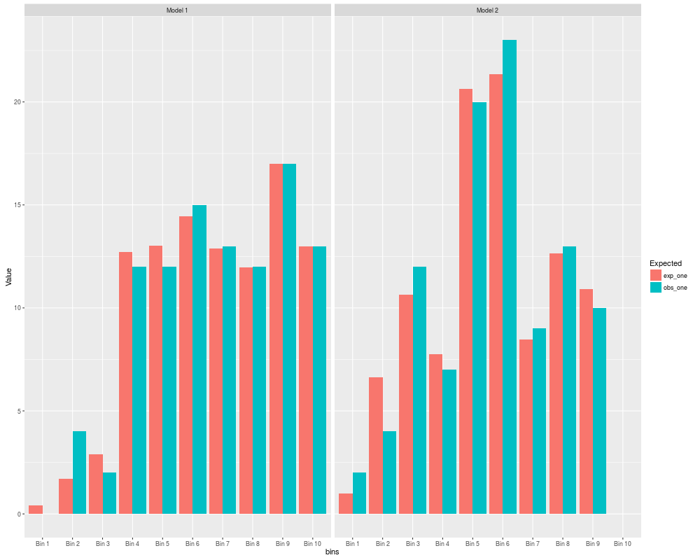
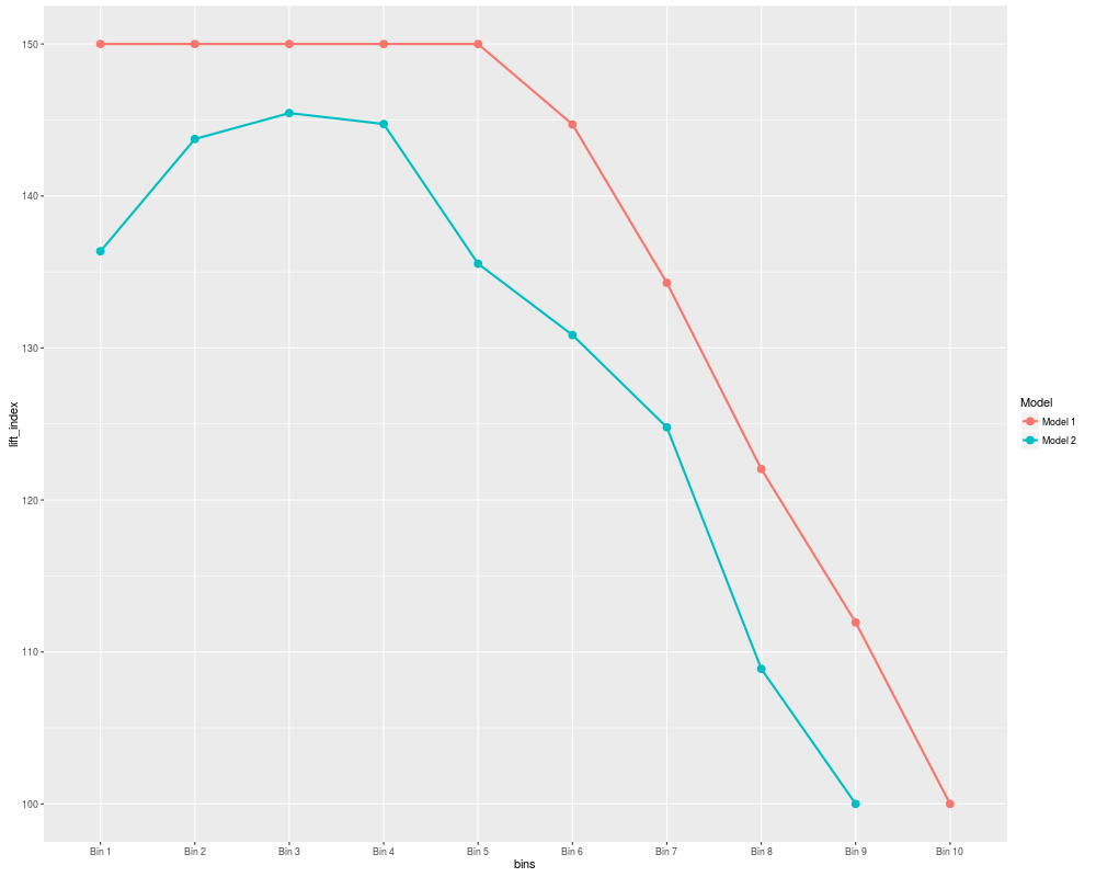
Generates & plots the following performance evaluation & validation measures for Binary Classification Models - Hosmer Lemeshow goodness of fit tests, Calibration plots, Lift index & gain charts & concordance-discordance measures

Usage

staticPerfMeasures(list_models, g, perf_measures = c("hosmer", "calibration",
  "lift", "concord"), sample_size_concord = 5000)

Arguments

`list_models`	A list of one (or more) dataframes for each model whose performance is to be evaluated. Each dataframe should comprise of 2 columns with the first column indicating the class labels (0 or 1) and the second column providing the raw predicted probabilities
`g`	The number of groups for binning. The predicted probabilities are binned as follows For Hosmer-Lemshow (HL) test: Predicted probabilities binned as per g unique quantiles i.e. cut_points = unique(quantile(predicted_prob,seq(0,1,1/g))) For Lift-Index & Gain charts: Same as HL test, however if g > unique(predicted_probability), the predicted probabilities are used as such without binning For calibration plots, g equal sized intervals are created (of width 1/g each)
`perf_measures`	Select the required performance evaluation and validation measure/s, from the following options - c('hosmer','calibration','lift','concord'). Default option is All
`sample_size_concord`	For computing concordance-discordance measures (and c-statistic) a random sample is drawn from each dataset (if nrow(dataset) > 5000). Default sample size of 5000 can be adjusted by changing the value of this argument

Value

A nested list with 2 components - a list of dataframes and a list of plots - containing the outcomes of the different performance evaluations carried out.

Examples

model_1 <- glm(Species ~ Sepal.Length,data=iris,family=binomial)
model_2 <- glm(Species ~ Sepal.Width, data=iris, family = binomial)
df1 <- data.frame(model_1$y,fitted(model_1))
df2 <- data.frame(model_2$y,fitted(model_2))
staticPerfMeasures(list(df1,df2),g=10, perf_measures = c("hosmer","lift"))

Results


R version 3.3.1 (2016-06-21) -- "Bug in Your Hair"
Copyright (C) 2016 The R Foundation for Statistical Computing
Platform: x86_64-pc-linux-gnu (64-bit)

R is free software and comes with ABSOLUTELY NO WARRANTY.
You are welcome to redistribute it under certain conditions.
Type 'license()' or 'licence()' for distribution details.

R is a collaborative project with many contributors.
Type 'contributors()' for more information and
'citation()' on how to cite R or R packages in publications.

Type 'demo()' for some demos, 'help()' for on-line help, or
'help.start()' for an HTML browser interface to help.
Type 'q()' to quit R.

> library(IMP)
> png(filename="/home/ddbj/snapshot/RGM3/R_CC/result/IMP/staticPerfMeasures.Rd_%03d_medium.png", width=480, height=480)
> ### Name: staticPerfMeasures
> ### Title: Model evaluation measures for Binary classification models
> ### Aliases: staticPerfMeasures
> 
> ### ** Examples
> 
> model_1 <- glm(Species ~ Sepal.Length,data=iris,family=binomial)
> model_2 <- glm(Species ~ Sepal.Width, data=iris, family = binomial)
> df1 <- data.frame(model_1$y,fitted(model_1))
> df2 <- data.frame(model_2$y,fitted(model_2))
> staticPerfMeasures(list(df1,df2),g=10, perf_measures = c("hosmer","lift"))
$data
$data$hosmer_df
     Model        cut_points obs_zero obs_one     exp_zero    exp_one
1  Model 1 [0.003785,0.0481]       16       0 1.559714e+01  0.4028642
2  Model 1   (0.0481,0.1246]       12       4 1.428553e+01  1.7144657
3  Model 1   (0.1246,0.3672]       11       2 1.012156e+01  2.8784398
4  Model 1   (0.3672,0.7605]        8      12 7.275105e+00 12.7248948
5  Model 1   (0.7605,0.8994]        3      12 1.968472e+00 13.0315280
6  Model 1   (0.8994,0.9769]        0      15 5.555367e-01 14.4444633
7  Model 1   (0.9769,0.9917]        0      13 1.307138e-01 12.8692862
8  Model 1   (0.9917,0.9973]        0      12 4.979819e-02 11.9502018
9  Model 1   (0.9973,0.9996]        0      17 1.543411e-02 16.9845659
10 Model 1        (0.9996,1]        0      13 7.096153e-04 12.9992904
11 Model 2    [0.0047,0.173]       13       2 1.401444e+01  0.9855620
12 Model 2     (0.173,0.362]       18       4 1.537659e+01  6.6234075
13 Model 2     (0.362,0.597]        7      12 8.371962e+00 10.6280384
14 Model 2     (0.597,0.705]        4       7 3.245361e+00  7.7546393
15 Model 2     (0.705,0.794]        6      20 5.352510e+00 20.6474903
16 Model 2      (0.794,0.91]        1      23 2.650112e+00 21.3498880
17 Model 2      (0.91,0.942]        0       9 5.223166e-01  8.4776834
18 Model 2     (0.942,0.977]        0      13 3.685488e-01 12.6314512
19 Model 2     (0.977,0.998]        1      10 9.816020e-02 10.9018398

$data$hosmer_results
    Model chi_square    p_value
1 Model 1    5.68090 0.68292584
2 Model 2   13.80271 0.08705474

$data$lift
     Model        cut_points cum_capture_1 fpr lift_index KS
1  Model 1        (0.9996,1]            13   0   150.0000 13
2  Model 1   (0.9973,0.9996]            30   0   150.0000 30
3  Model 1   (0.9917,0.9973]            42   0   150.0000 42
4  Model 1   (0.9769,0.9917]            55   0   150.0000 55
5  Model 1   (0.8994,0.9769]            70   0   150.0000 70
6  Model 1   (0.7605,0.8994]            82   6   144.7059 76
7  Model 1   (0.3672,0.7605]            94  22   134.2857 72
8  Model 1   (0.1246,0.3672]            96  44   122.0339 52
9  Model 1   (0.0481,0.1246]           100  68   111.9403 32
10 Model 1 [0.003785,0.0481]           100 100   100.0000  0
11 Model 2     (0.977,0.998]            10   2   136.3636  8
12 Model 2     (0.942,0.977]            23   2   143.7500 21
13 Model 2      (0.91,0.942]            32   2   145.4545 30
14 Model 2      (0.794,0.91]            55   4   144.7368 51
15 Model 2     (0.705,0.794]            75  16   135.5422 59
16 Model 2     (0.597,0.705]            82  24   130.8511 58
17 Model 2     (0.362,0.597]            94  38   124.7788 56
18 Model 2     (0.173,0.362]            98  74   108.8889 24
19 Model 2    [0.0047,0.173]           100 100   100.0000  0


$plots
$plots$hosmer

$plots$lift


> 
> 
> 
> 
> 
> dev.off()
null device 
          1 
>