Supported by Dr. Osamu Ogasawara and  . . |
|
Last data update: 2014.03.03 |
NSS.JD Method for Nonstationary Blind Source SeparationDescriptionThe NSS.JD method for nonstationary blind source separation. The method first whitens the complete data and then divides it into K time intervals.
Then UsageNSS.JD(X, ...) ## Default S3 method: NSS.JD(X, K=12, Tau=0, n.cuts=NULL, eps = 1e-06, maxiter = 100, ...) ## S3 method for class 'ts' NSS.JD(X, ...) Arguments
DetailsThe model assumes that the mean of the p-variate time series is constant but the variances change over time. ValueA list with class 'bss' containing the following components:
Author(s)Klaus Nordhausen ReferencesChoi S. and Cichocki A. (2000), Blind separation of nonstationary sources in noisy mixtures, Electronics Letters, 36, 848–849. Choi S. and Cichocki A. (2000), Blind separation of nonstationary and temporally correlated sources from noisy mixtures, Proceedings of the 2000 IEEE Signal Processing Society Workshop Neural Networks for Signal Processing X, 1, 405–414. Nordhausen K. (2013), On robustifying some second order blind source separation methods for nonstationary time series, to appear in Statistical Papers, ??, ???–???. See Also
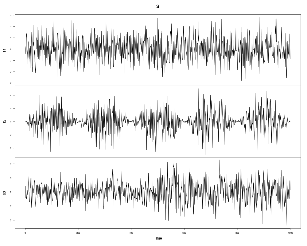
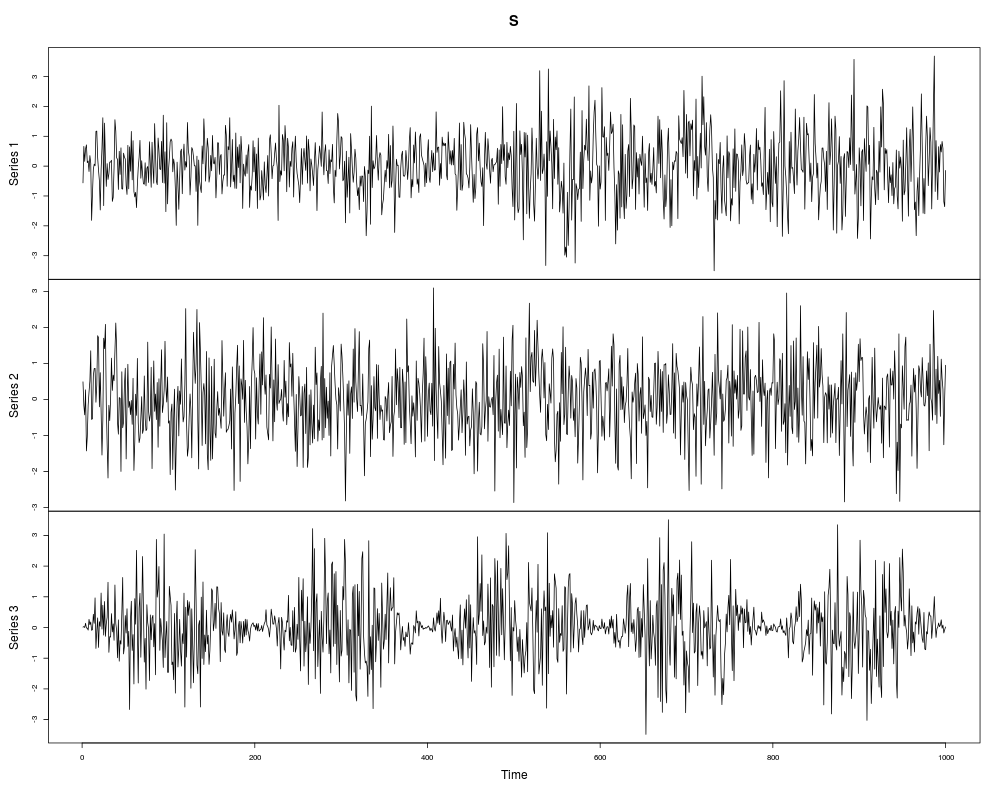
Examplesn <- 1000 s1 <- rnorm(n) s2 <- 2*sin(pi/200*1:n)* rnorm(n) s3 <- c(rnorm(n/2), rnorm(100,0,2), rnorm(n/2-100,0,1.5)) S <- cbind(s1,s2,s3) plot.ts(S) A<-matrix(rnorm(9),3,3) X<- S%*%t(A) NSS2 <- NSS.JD(X) NSS2 MD(coef(NSS2),A) plot(NSS2) cor(NSS2$S,S) NSS2b <- NSS.JD(X, Tau=1) MD(coef(NSS2b),A) NSS2c <- NSS.JD(X, n.cuts=c(1,300,500,600,1000)) MD(coef(NSS2c),A) Results
R version 3.3.1 (2016-06-21) -- "Bug in Your Hair"
Copyright (C) 2016 The R Foundation for Statistical Computing
Platform: x86_64-pc-linux-gnu (64-bit)

R is free software and comes with ABSOLUTELY NO WARRANTY.
You are welcome to redistribute it under certain conditions.
Type 'license()' or 'licence()' for distribution details.

R is a collaborative project with many contributors.
Type 'contributors()' for more information and
'citation()' on how to cite R or R packages in publications.

Type 'demo()' for some demos, 'help()' for on-line help, or
'help.start()' for an HTML browser interface to help.
Type 'q()' to quit R.

> library(JADE)
> png(filename="/home/ddbj/snapshot/RGM3/R_CC/result/JADE/NSS.JD.Rd_%03d_medium.png", width=480, height=480)
> ### Name: NSS.JD
> ### Title: NSS.JD Method for Nonstationary Blind Source Separation
> ### Aliases: NSS.JD NSS.JD.default NSS.JD.ts
> ### Keywords: multivariate ts
>
> ### ** Examples
>
> n <- 1000
> s1 <- rnorm(n)
> s2 <- 2*sin(pi/200*1:n)* rnorm(n)
> s3 <- c(rnorm(n/2), rnorm(100,0,2), rnorm(n/2-100,0,1.5))
> S <- cbind(s1,s2,s3)
> plot.ts(S)
> A<-matrix(rnorm(9),3,3)
> X<- S%*%t(A)
>
> NSS2 <- NSS.JD(X)
> NSS2
W :
          [,1]      [,2]        [,3]
[1,] 0.7696092 0.2337227  1.40683275
[2,] 0.2479964 0.5308625 -0.03525854
[3,] 0.2200833 0.4107085  2.49981387

k :
[1] 0

n.cut :
 [1]    1   85  168  251  334  418  501  584  667  751  834  917 1000

K :
[1] 12

> MD(coef(NSS2),A)
[1] 0.08784887
> plot(NSS2)
> cor(NSS2$S,S)
                  s1          s2         s3
Series 1 -0.03013461 -0.99773152 0.07970551
Series 2  0.04035608  0.04475109 0.99660604
Series 3 -0.99873084  0.05029066 0.02057730
>
> NSS2b <- NSS.JD(X, Tau=1)
> MD(coef(NSS2b),A)
[1] 0.850378
>
> NSS2c <- NSS.JD(X, n.cuts=c(1,300,500,600,1000))
> MD(coef(NSS2c),A)
[1] 0.6867715
>
>
>
>
>
> dev.off()
null device
          1
>
|