R Graphical Manual

Browse All

Last data update: 2014.03.03

R: SOBI Method for Blind Source Separation

SOBI	R Documentation

SOBI Method for Blind Source Separation

Description

The SOBI method for the second order blind source separation problem. The function estimates the unmixing matrix in a second order stationary source separation model by jointly diagonalizing the covariance matrix and several autocovariance matrices at different lags.

Usage

SOBI(X, ...)

## Default S3 method:
SOBI(X, k=12, method="frjd", eps = 1e-06, maxiter = 100, ...)
## S3 method for class 'ts'
SOBI(X, ...)

Arguments

`X`	a numeric matrix or a multivariate time series object of class `ts`. Missing values are not allowed.
`k`	if a single integer, then the lags 1:k are used, if an integer vector, then these are used as the lags.
`method`	method to use for the joint diagonalization, options are `djd`, `rjd` and `frjd`

`eps`	maximum number of iterations.
`maxiter`	convergence tolerance.
`...`	further arguments to be passed to or from methods.

Details

The order of the estimated components is fixed so that the sums of squared autocovariances are in the decreasing order.

Value

A list with class 'bss' containing the following components:

`W`	estimated unmixing matrix.
`k`	lags used.
`method`	method used for the joint diagonalization.
`S`	estimated sources as time series objected standardized to have mean 0 and unit variances.

Author(s)

Klaus Nordhausen

References

Belouchrani, A., Abed-Meriam, K., Cardoso, J.F. and Moulines, R. (1997), A blind source separation technique using second-order statistics, IEEE Transactions on Signal Processing, 434–444.

Miettinen, J., Nordhausen, K., Oja, H. and Taskinen, S. (2013), Deflation-based Separation of Uncorrelated Stationary Time Series, Journal of Multivariate Analysis, ??, ???–???.

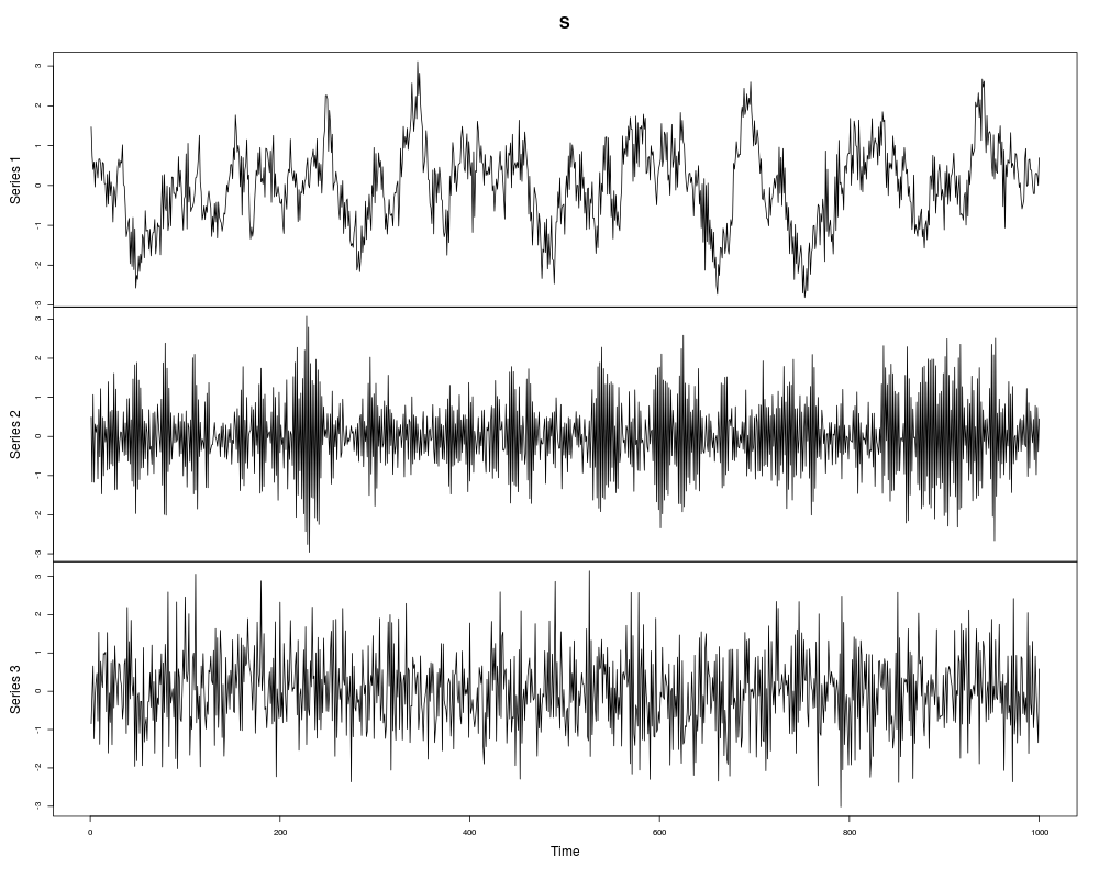
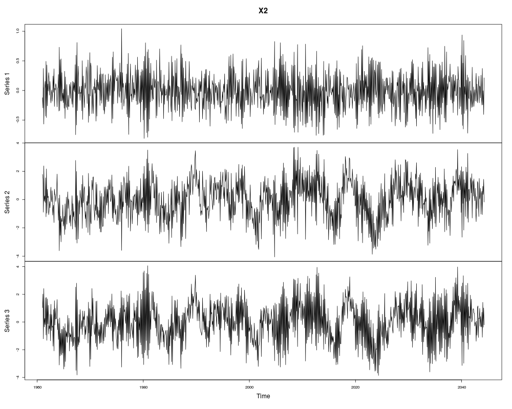
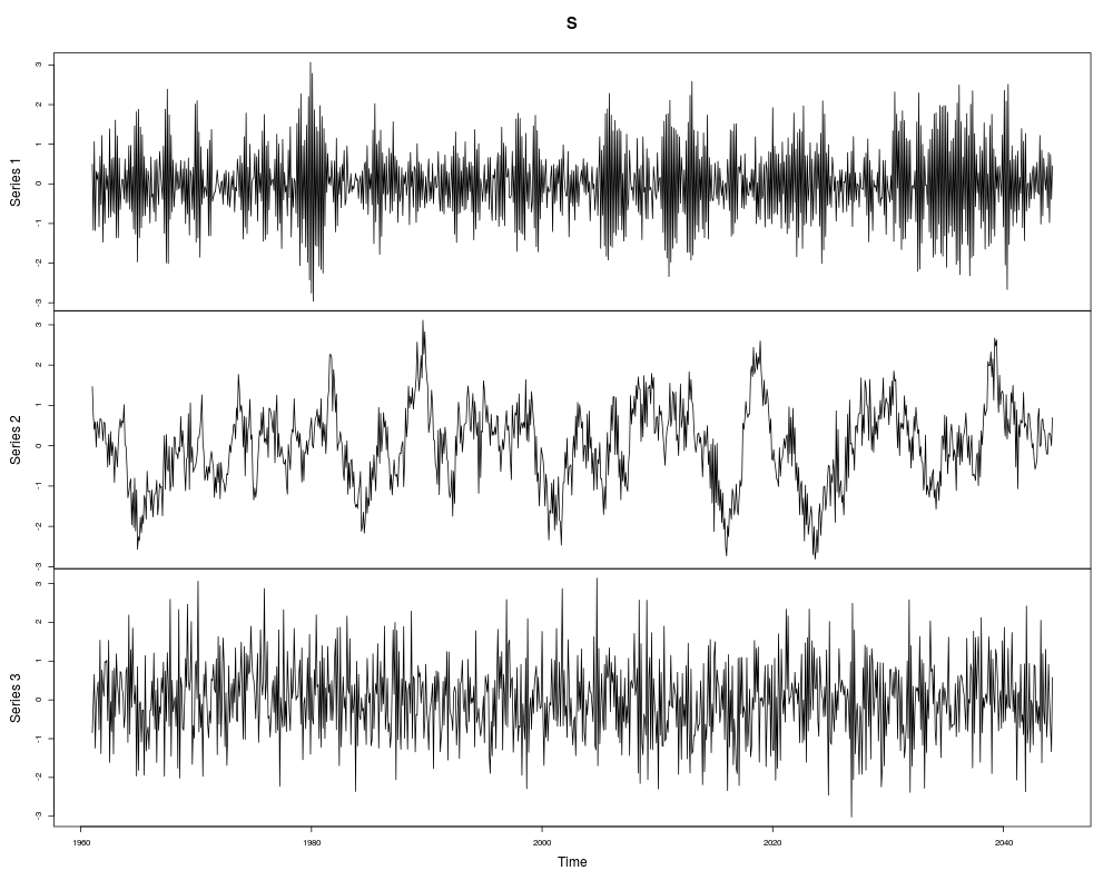
Examples

# creating some toy data
A<- matrix(rnorm(9),3,3)
s1 <- arima.sim(list(ar=c(0.3,0.6)),1000)
s2 <- arima.sim(list(ma=c(-0.3,0.3)),1000)
s3 <- arima.sim(list(ar=c(-0.8,0.1)),1000)

S <- cbind(s1,s2,s3)
X <- S %*% t(A)

res1<-SOBI(X)
res1
coef(res1)
plot(res1) # compare to plot.ts(S)
MD(coef(res1),A)

# input of a time series
X2<- ts(X, start=c(1961, 1), frequency=12)
plot(X2)
res2<-SOBI(X2, k=c(5,10,1,4,2,9,10))
plot(res2)

Results


R version 3.3.1 (2016-06-21) -- "Bug in Your Hair"
Copyright (C) 2016 The R Foundation for Statistical Computing
Platform: x86_64-pc-linux-gnu (64-bit)

R is free software and comes with ABSOLUTELY NO WARRANTY.
You are welcome to redistribute it under certain conditions.
Type 'license()' or 'licence()' for distribution details.

R is a collaborative project with many contributors.
Type 'contributors()' for more information and
'citation()' on how to cite R or R packages in publications.

Type 'demo()' for some demos, 'help()' for on-line help, or
'help.start()' for an HTML browser interface to help.
Type 'q()' to quit R.

> library(JADE)
> png(filename="/home/ddbj/snapshot/RGM3/R_CC/result/JADE/SOBI.Rd_%03d_medium.png", width=480, height=480)
> ### Name: SOBI
> ### Title: SOBI Method for Blind Source Separation
> ### Aliases: SOBI SOBI.default SOBI.ts
> ### Keywords: multivariate ts
> 
> ### ** Examples
> 
> # creating some toy data
> A<- matrix(rnorm(9),3,3)
> s1 <- arima.sim(list(ar=c(0.3,0.6)),1000)
> s2 <- arima.sim(list(ma=c(-0.3,0.3)),1000)
> s3 <- arima.sim(list(ar=c(-0.8,0.1)),1000)
> 
> S <- cbind(s1,s2,s3)
> X <- S %*% t(A)
> 
> res1<-SOBI(X)
> res1
W :
           [,1]        [,2]       [,3]
[1,] 0.31072690 -0.01098166  0.1591190
[2,] 0.09067729  0.34217640 -0.2260787
[3,] 0.02502008  0.43605431  0.3255149

k :
 [1]  1  2  3  4  5  6  7  8  9 10 11 12

method :
[1] "frjd"

> coef(res1)
           [,1]        [,2]       [,3]
[1,] 0.31072690 -0.01098166  0.1591190
[2,] 0.09067729  0.34217640 -0.2260787
[3,] 0.02502008  0.43605431  0.3255149
> plot(res1) # compare to plot.ts(S)
> MD(coef(res1),A)
[1] 0.03342505
> 
> # input of a time series
> X2<- ts(X, start=c(1961, 1), frequency=12)
> plot(X2)
> res2<-SOBI(X2, k=c(5,10,1,4,2,9,10))
> plot(res2)
> 
> 
> 
> 
> 
> dev.off()
null device 
          1 
>