Supported by Dr. Osamu Ogasawara and  . . |
|
Last data update: 2014.03.03 |
Plot Method for survfitJM ObjectsDescriptionProduces plots of conditional probabilities of survival. Usage
## S3 method for class 'survfitJM'
plot(x, estimator = c("both", "mean", "median"),
    which = NULL, fun = NULL, conf.int = FALSE,
    fill.area = FALSE, col.area = "grey", col.abline = "black", col.points = "black",
    add.last.time.axis.tick = FALSE, include.y = FALSE, main = NULL,
    xlab = NULL, ylab = NULL, ylab2 = NULL, lty = NULL, col = NULL,
    lwd = NULL, pch = NULL, ask = NULL, legend = FALSE, ...,
    cex.axis.z = 1, cex.lab.z = 1)
Arguments
Author(s)Dimitris Rizopoulos d.rizopoulos@erasmusmc.nl ReferencesRizopoulos, D. (2012) Joint Models for Longitudinal and Time-to-Event Data: with Applications in R. Boca Raton: Chapman and Hall/CRC. Rizopoulos, D. (2011). Dynamic predictions and prospective accuracy in joint models for longitudinal and time-to-event data. Biometrics 67, 819–829. Rizopoulos, D. (2010) JM: An R Package for the Joint Modelling of Longitudinal and Time-to-Event Data. Journal of Statistical Software 35 (9), 1–33. http://www.jstatsoft.org/v35/i09/ See Also
Examples
# linear mixed model fit
fitLME <- lme(sqrt(CD4) ~ obstime + obstime:drug,
random = ~ 1 | patient, data = aids)
# cox model fit
fitCOX <- coxph(Surv(Time, death) ~ drug, data = aids.id, x = TRUE)
# joint model fit
fitJOINT <- jointModel(fitLME, fitCOX,
timeVar = "obstime", method = "weibull-PH-aGH")
# sample of the patients who are still alive
ND <- aids[aids$patient == "141", ]
ss <- survfitJM(fitJOINT, newdata = ND, idVar = "patient", M = 50)
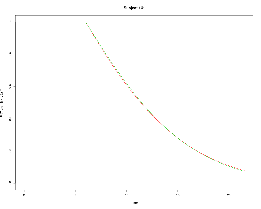
plot(ss)
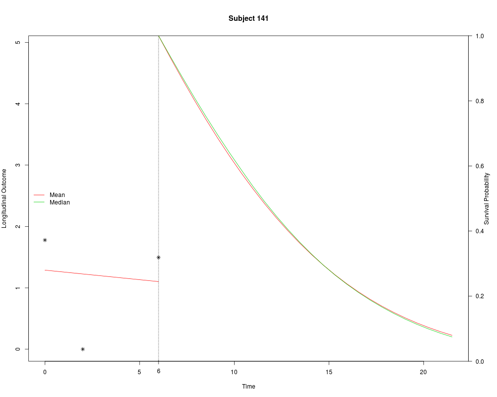
plot(ss, include.y = TRUE, add.last.time.axis.tick = TRUE, legend = TRUE)
Results
R version 3.3.1 (2016-06-21) -- "Bug in Your Hair"
Copyright (C) 2016 The R Foundation for Statistical Computing
Platform: x86_64-pc-linux-gnu (64-bit)

R is free software and comes with ABSOLUTELY NO WARRANTY.
You are welcome to redistribute it under certain conditions.
Type 'license()' or 'licence()' for distribution details.

R is a collaborative project with many contributors.
Type 'contributors()' for more information and
'citation()' on how to cite R or R packages in publications.

Type 'demo()' for some demos, 'help()' for on-line help, or
'help.start()' for an HTML browser interface to help.
Type 'q()' to quit R.

> library(JM)
Loading required package: MASS
Loading required package: nlme
Loading required package: splines
Loading required package: survival
> png(filename="/home/ddbj/snapshot/RGM3/R_CC/result/JM/plot-survfitJM.Rd_%03d_medium.png", width=480, height=480)
> ### Name: plot.survfitJM
> ### Title: Plot Method for survfitJM Objects
> ### Aliases: plot.survfitJM
> ### Keywords: methods
>
> ### ** Examples
>
> # linear mixed model fit
> fitLME <- lme(sqrt(CD4) ~ obstime + obstime:drug,
+     random = ~ 1 | patient, data = aids)
> # cox model fit
> fitCOX <- coxph(Surv(Time, death) ~ drug, data = aids.id, x = TRUE)
>
> # joint model fit
> fitJOINT <- jointModel(fitLME, fitCOX,
+     timeVar = "obstime", method = "weibull-PH-aGH")
>
> # sample of the patients who are still alive
> ND <- aids[aids$patient == "141", ]
> ss <- survfitJM(fitJOINT, newdata = ND, idVar = "patient", M = 50)
> plot(ss)
> plot(ss, include.y = TRUE, add.last.time.axis.tick = TRUE, legend = TRUE)
>
>
>
>
>
> dev.off()
null device
          1
>
|