Displaying the Joint Optimization Plot

Description

The function plot.JOP takes the output produced by JOP and returns the joint optimization plot.

Usage

## S3 method for class 'JOP'
plot(x, no.col = FALSE, standard = TRUE, col = 1, lty = 1, bty = "l",
las = 1 ,adj = 0.5 ,cex = 1 ,cex.lab = 1 ,cex.axis = 1,
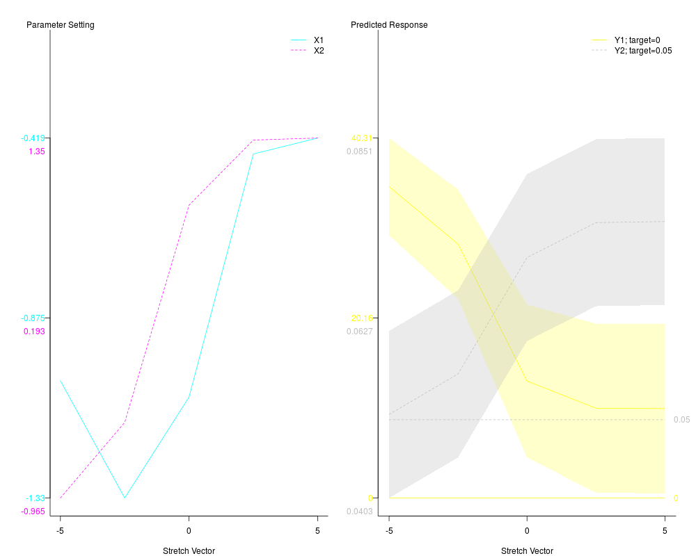
xlab = c("Stretch Vector" , "Stretch Vector"),
ylab = c("Parameter Setting" , "Predicted Response"),lwd=1,...)

Arguments

Details

Let nx be the number of parameters (number of columns of datax) and ny be the number of responses (number of columns of datay). Then col and lty must have length nx+ny. Otherwise predefined grey colors (for no.col=TRUE) or standard colors 1, 2, ..., nx+ny are used. The arguments xlab and ylab must have length two, where the first entry contains the label for x-axis and y-axis of the left hand plot and the second entry contains the label for x-axis and y-axis of the right hand plot. Additional graphical arguments can be plugged in.

References

Sonja Kuhnt and Martina Erdbruegge (2004). A strategy of robust paramater design for multiple responses, Statistical Modelling; 4: 249-264, TU Dortmund.

Martina Erdbruegge, Sonja Kuhnt and Nikolaus Rudak (2011). Joint optimization of independent multiple responses based on loss functions, Quality and Reliability Engineering International 27, doi: 10.1002/qre.1229.

Joseph J. Pignatiello (1993). Strategies for robust multiresponse quality engineering, IIE Transactions 25, 5-15, Texas A M University.

Alexios Ghalanos and Stefan Theussl (2012). Rsolnp: General Non-linear Optimization Using Augmented Lagrange Multiplier Method. R package version 1.12.

Peter K Dunn and Gordon K Smyth (2012). dglm: Double generalized linear models, R package version 1.6.2.

Sonja Kuhnt, Nikolaus Rudak (2013). Simultaneous Optimization of Multiple Responses with the R Package JOP, Journal of Statistical Software, 54(9), 1-23, URL http://www.jstatsoft.org/v54/i09/.

Examples

# Example: Sheet metal hydroforming process
outtest <- JOP(datax = datax, datay = datay, tau = list(0 , 0.05), numbW = 5)

# Several graphical parameters can be plugged in
plot(outtest, col = 5:8)

Results

R version 3.3.1 (2016-06-21) -- "Bug in Your Hair"
Copyright (C) 2016 The R Foundation for Statistical Computing
Platform: x86_64-pc-linux-gnu (64-bit)

R is free software and comes with ABSOLUTELY NO WARRANTY.
You are welcome to redistribute it under certain conditions.
Type 'license()' or 'licence()' for distribution details.

R is a collaborative project with many contributors.
Type 'contributors()' for more information and
'citation()' on how to cite R or R packages in publications.

Type 'demo()' for some demos, 'help()' for on-line help, or
'help.start()' for an HTML browser interface to help.
Type 'q()' to quit R.

> library(JOP)
Loading required package: Rsolnp
Loading required package: dglm
Loading required package: statmod
> png(filename="/home/ddbj/snapshot/RGM3/R_CC/result/JOP/plot.JOP.rd_%03d_medium.png", width=480, height=480)
> ### Name: plot.JOP
> ### Title: Displaying the Joint Optimization Plot
> ### Aliases: plot.JOP
> 
> ### ** Examples
> 
> # Example: Sheet metal hydroforming process
> outtest <- JOP(datax = datax, datay = datay, tau = list(0 , 0.05), numbW = 5)
Automatic Modeling starts...

Model building finished ....
 
Cost matrices calculated ....
 
Optimization starts ....
    |                                                                               |                                                                      |   0%   |                                                                               |==============                                                        |  20%   |                                                                               |============================                                          |  40%   |                                                                               |==========================================                            |  60%   |                                                                               |========================================================              |  80%   |                                                                               |======================================================================| 100%
Optimization finished ....
 
> 
> # Several graphical parameters can be plugged in
> plot(outtest, col = 5:8)
> 
> 
> 
> 
> 
> dev.off()
null device 
          1 
>