Supported by Dr. Osamu Ogasawara and  . . |
|
Last data update: 2014.03.03 |
Provides functions for some small area estimators and their variances (mean squared errors).DescriptionThis package currently implements the unit level EBLUP (Battese et al. 1988) and GREG (Sarndal 1984) estimators as well as their variance estimators. It also contains data and a vignette that explain its use. DetailsThe aim in the analysis of sample surveys is frequently to derive estimates of subpopulation characteristics. Often, the sample available for the subpopulation is, however, too small to allow a reliable estimate. If an auxiliary variable exists that is correlated with the variable of interest, small area estimation (SAE) provides methods to solve the problem (Rao 2003). The purpose of this package is primarily to document the functions used in the publications Breidenbach and Astrup (2012). The data used in that study are also provided. The vignette further documents the publication Breidenbach et al. (2015). You might wonder why this package is called JoSAE. Well, first of all, JoSAE sounds good (if pronounced like the female name). The other reason was that the packages SAE and SAE2 already exist (Gomez-Rubio, 2008). They are, however, not available on CRAN and unmaintained (as of July 2011). They also do not seem to implement the variance estimators that we needed. So I just combined SAE with the first part of my name. NoteAll the implemented functions/estimators are described in Rao (2003). This package merely makes the use of the estimators easier for the users that are not keen on programming. Especially the EBLUP variance estimator would require some effort. Today, there are several well programmed SAE packages available on CRAN that also provide the functions described here. This was not the case when the first version of the package was uploaded. This package is therefore mostly to document the publications mentioned above. There are several points where the JoSAE package could be improved: Only univariate unit-level models with a simple block-diagonal variance structure are supported so far. The computation is based on loops on the domain level. It would be more elegant to use blocked matrices. ... many more things ... Author(s)Johannes Breidenbach Maintainer: Johannes Breidenbach <job@nibio.no> ReferencesBattese, G. E., Harter, R. M. & Fuller, W. A. (1988), An error-components model for prediction of county crop areas using survey and satellite data Journal of the American Statistical Association, 83, 28-36 Breidenbach, J. and Astrup, R. (2012), Small area estimation of forest attributes in the Norwegian National Forest Inventory. European Journal of Forest Research, 131:1255-1267. Breidenbach, J., Ronald E. McRoberts, Astrup, R. (2015), Empirical coverage of model-based variance estimators for remote sensing assisted estimation of stand-level timber volume. Remote Sensing of Environment. In press. Gomez-Rubio (2008), Tutorial on small area estimation, UseR conference 2008, August 12-14, Technische Universitat Dortmund, Germany. Rao, J.N.K. (2003), Small area estimation. Wiley. Sarndal, C. (1984), Design-consistent versus model-dependent estimation for small domains Journal of the American Statistical Association, JSTOR, 624-631 Schoch, T. (2011), rsae: Robust Small Area Estimation. R package version 0.1-3. See Also
Examples
#mean auxiliary variables for the populations in the domains
data(JoSAE.domain.data)
#data for the sampled elements
data(JoSAE.sample.data)
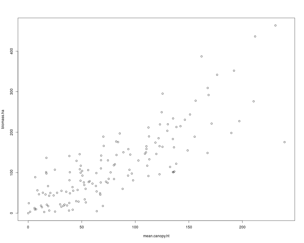
plot(biomass.ha~mean.canopy.ht,JoSAE.sample.data)
## the easy way: use the wrapper function to compute EBLUP and GREG estimates and variances
#lme model
summary(fit.lme <- lme(biomass.ha ~ mean.canopy.ht, data=JoSAE.sample.data
, random=~1|domain.ID))
#domain data need to have the same column names as sample data or vice versa
d.data <- JoSAE.domain.data
names(d.data)[3] <- "mean.canopy.ht"
result <- eblup.mse.f.wrap(domain.data = d.data, lme.obj = fit.lme)
result
##END: the easy way
##the hard way: compute the EBLUP MSE components yourself
#get an overview of the domains
#mean of the response and predictor variables from the sample.
#For the response this is the sample mean estimator.
tmp <- aggregate(JoSAE.sample.data[,c("biomass.ha", "mean.canopy.ht")]
, by=list(domain.ID=JoSAE.sample.data$domain.ID), mean)
names(tmp)[2:3] <- paste(names(tmp)[2:3], ".bar.sample", sep="")
#number of samples within the domains
tmp1 <- aggregate(cbind(n.i=JoSAE.sample.data$biomass.ha)
, by=list(domain.ID=JoSAE.sample.data$domain.ID), length)
#combine it with the population information of the domains
overview.domains <- cbind(JoSAE.domain.data, tmp[,-1], n.i=tmp1[,-1])
#fit the models
#lm - the auxiliary variable explains forest biomass rather good
summary(fit.lm <- lm(biomass.ha ~ mean.canopy.ht, data=JoSAE.sample.data))
#lme
summary(fit.lme <- lme(biomass.ha ~ mean.canopy.ht, data=JoSAE.sample.data
, random=~1|domain.ID))
#mean lm residual -- needed for GREG
overview.domains$mean.resid.lm <- aggregate(resid(fit.lm)
, by=list(domain.ID=JoSAE.sample.data$domain.ID)
, mean)[,2]
#mean lme residual -- needed for EBLUP.var
overview.domains$mean.resid.lme <- aggregate(resid(fit.lme, level=0)
, by=list(domain.ID=JoSAE.sample.data$domain.ID)
, mean)[,2]
#synthetic estimate
overview.domains$synth <- predict(fit.lm
, newdata= data.frame(mean.canopy.ht=JoSAE.domain.data$mean.canopy.ht.bar))
#GREG estimate
overview.domains$GREG <- overview.domains$synth + overview.domains$mean.resid.lm
#EBLUP estimate
overview.domains$EBLUP <- predict(fit.lme
, newdata=data.frame(mean.canopy.ht=JoSAE.domain.data$mean.canopy.ht.bar
, domain.ID=JoSAE.domain.data$domain.ID)
, level=1)
#gamma
overview.domains$gamma.i <- eblup.mse.f.gamma.i(lme.obj=fit.lme
, n.i=overview.domains$n.i)
#variance of the sample mean estimate
overview.domains$sample.var <-
aggregate(JoSAE.sample.data$biomass.ha
, by=list(domain.ID=JoSAE.sample.data$domain.ID), var)[,-1]/overview.domains$n.i
#variance of the GREG estimate
overview.domains$GREG.var <-
aggregate(resid(fit.lm)
, by=list(domain.ID=JoSAE.sample.data$domain.ID),var)[,-1]/overview.domains$n.i
#variance of the EBLUP
#compute the A.i matrices for all domains (only needed once)
domain.ID <- JoSAE.domain.data$domain.ID
#initialize the result vector
a.i.mats <- vector(mode="list", length=length(domain.ID))
for(i in 1:length(domain.ID)){
print(i)
a.i.mats[[i]] <- eblup.mse.f.c2.ai(gamma.i=overview.domains$gamma.i[
overview.domains$domain.ID==domain.ID[i]]
, n.i=overview.domains$n.i[overview.domains$domain.ID==domain.ID[i]]
, lme.obj=fit.lme
, X.i=as.matrix(cbind(i=1
, x=JoSAE.sample.data[JoSAE.sample.data$domain.ID==domain.ID[i], "mean.canopy.ht"]
))
)
}
#add all the matrices
sum.A.i.mats <- Reduce("+", a.i.mats)
#the assymptotic var-cov matrix
asy.var.cov.mat <- eblup.mse.f.c3.asyvarcovarmat(n.i=overview.domains$n.i
, lme.obj=fit.lme)
#put together the variance components
###### Some changes are required here, if you apply it to own data!
result <- NULL
for(i in 1:length(domain.ID)){
print(i)
#first comp
mse.c1.tmp <- eblup.mse.f.c1(gamma.i=overview.domains$gamma.i[
overview.domains$domain.ID==domain.ID[i]]
, n.i=overview.domains$n.i[overview.domains$domain.ID==domain.ID[i]]
, lme.obj=fit.lme)
#second comp
mse.c2.tmp <- eblup.mse.f.c2(gamma.i=overview.domains$gamma.i[
overview.domains$domain.ID==domain.ID[i]]
, X.i=as.matrix(cbind(i=1##cbind!!
, x=JoSAE.sample.data[JoSAE.sample.data$domain.ID==domain.ID[i]
, "mean.canopy.ht"]##change to other varnames if necessary
))
, X.bar.i =as.matrix(rbind(i=1##rbind!!
, x=JoSAE.domain.data[JoSAE.domain.data$domain.ID==domain.ID[i]
, "mean.canopy.ht.bar"]##change to other varnames if necessary
))
, sum.A.i = sum.A.i.mats
)
#third comp
mse.c3.tmp <- eblup.mse.f.c3(n.i=overview.domains$n.i[
overview.domains$domain.ID==domain.ID[i]]
, lme.obj=fit.lme
, asympt.var.covar=asy.var.cov.mat)
#third star comp
mse.c3.star.tmp <- eblup.mse.f.c3.star( n.i=overview.domains$n.i[
overview.domains$domain.ID==domain.ID[i]]
, lme.obj=fit.lme
, mean.resid.i=overview.domains$mean.resid.lme[
overview.domains$domain.ID==domain.ID[i]]
, asympt.var.covar=asy.var.cov.mat)
#save result
result <- rbind(result, data.frame(kommune=domain.ID[i]
, n.i=overview.domains$n.i[overview.domains$domain.ID==domain.ID[i]]
, c1=as.numeric(mse.c1.tmp), c2=as.numeric(mse.c2.tmp)
, c3=as.numeric(mse.c3.tmp), c3star=as.numeric(mse.c3.star.tmp)))
}
#derive the actual EBLUP variances
overview.domains$EBLUP.var.1 <- result$c1 + result$c2 + 2* result$c3star
overview.domains$EBLUP.var.2 <- result$c1 + result$c2 + result$c3 + result$c3star
#display the estimates and the sampling error (sqrt(var)) in two tables
round(data.frame(overview.domains[,c("domain.ID", "n.i", "N.i")],
overview.domains[,c("biomass.ha.bar.sample", "GREG", "synth", "EBLUP")]),2)
#the sampling errors of the eblup is mostly smaller than the one of the greg estimate.
#both are always smaller than the sample mean variance.
round(data.frame(overview.domains[,c("domain.ID", "n.i", "N.i")],
sqrt(overview.domains[,c("sample.var", "GREG.var",
"EBLUP.var.1", "EBLUP.var.2")])),2)
##END: the hard way
Results
R version 3.3.1 (2016-06-21) -- "Bug in Your Hair"
Copyright (C) 2016 The R Foundation for Statistical Computing
Platform: x86_64-pc-linux-gnu (64-bit)

R is free software and comes with ABSOLUTELY NO WARRANTY.
You are welcome to redistribute it under certain conditions.
Type 'license()' or 'licence()' for distribution details.

R is a collaborative project with many contributors.
Type 'contributors()' for more information and
'citation()' on how to cite R or R packages in publications.

Type 'demo()' for some demos, 'help()' for on-line help, or
'help.start()' for an HTML browser interface to help.
Type 'q()' to quit R.

> library(JoSAE)
Loading required package: nlme
> png(filename="/home/ddbj/snapshot/RGM3/R_CC/result/JoSAE/JoSAE-package.Rd_%03d_medium.png", width=480, height=480)
> ### Name: JoSAE-package
> ### Title: Provides functions for some small area estimators and their
> ###   variances (mean squared errors).
> ### Aliases: JoSAE-package JoSAE
> ### Keywords: package
>
> ### ** Examples
>
> 	#mean auxiliary variables for the populations in the domains
> data(JoSAE.domain.data)
> 	#data for the sampled elements
> data(JoSAE.sample.data)
> plot(biomass.ha~mean.canopy.ht,JoSAE.sample.data)
>
> ## the easy way: use the wrapper function to compute EBLUP and GREG estimates and variances
>
>     #lme model
> summary(fit.lme <- lme(biomass.ha ~ mean.canopy.ht, data=JoSAE.sample.data
+                        , random=~1|domain.ID))
Linear mixed-effects model fit by REML
 Data: JoSAE.sample.data
       AIC      BIC    logLik
  1553.764 1565.616 -772.8822

Random effects:
 Formula: ~1 | domain.ID
        (Intercept) Residual
StdDev:    10.30361 49.85829

Fixed effects: biomass.ha ~ mean.canopy.ht
                  Value Std.Error  DF   t-value p-value
(Intercept)    6.694678  8.334032 130  0.803294  0.4233
mean.canopy.ht 1.375782  0.077531 130 17.744832  0.0000
 Correlation:
               (Intr)
mean.canopy.ht -0.754

Standardized Within-Group Residuals:
        Min          Q1         Med          Q3         Max
-3.12149463 -0.56323615 -0.05238025  0.55696863  3.11427777

Number of Observations: 145
Number of Groups: 14
>
>     #domain data need to have the same column names as sample data or vice versa
> d.data <- JoSAE.domain.data
> names(d.data)[3] <- "mean.canopy.ht"
>
> result <- eblup.mse.f.wrap(domain.data = d.data, lme.obj = fit.lme)
> result
   domain.ID N.i.domain mean.canopy.ht.domain biomass.ha.sample.mean
1          1     105267             108.15832               92.72626
2          2     202513              77.34845              109.06437
3          3     134156              94.26035              169.54391
4          4     193807              86.64053               53.29122
5          5    1379945              84.87776              118.39030
6          6     176731              77.66091               93.62950
7          7     474615              71.40756              152.52385
8          8     442280              65.50692              106.39617
9          9     495568              81.65170              113.69878
10        10     520141              80.04376              124.13538
11        11     230756              92.17368              152.94990
12        12      83441              82.38918               34.10600
13        13      57858              63.28690              130.78382
14        14     905387              66.04283               97.76514
   mean.canopy.ht.sample.mean n.i.sample mean.resid.lm mean.resid.lme     Synth
1                    93.27877          1    -42.756667     -42.299623 155.73097
2                    93.24650          6    -26.374651     -25.917124 113.80502
3                   141.63208          3    -31.738017     -32.005579 136.81867
4                    52.49564          2    -26.694199     -25.625994 126.44965
5                    87.22426         35     -8.853691      -8.305917 124.05088
6                    46.39423          4     21.946850      23.106488 114.23021
7                    83.88586         17     29.822744      30.420546 105.72069
8                    65.95093         12      8.100855       8.967424  97.69111
9                    82.46554         12     -7.069557      -6.450470 119.66087
10                   97.12918         14    -16.587178     -16.187835 117.47278
11                   99.50661          8      8.992147       9.355863 133.97913
12                   52.80381          1    -46.298778     -45.235192 120.66442
13                   68.01002          1     29.686497      30.522209  94.67012
14                   59.75254         29      7.904559       8.864014  98.42038
       EBLUP      GREG    gamma.i sample.var.mean GREG.var.mean        c1
1  153.76439 112.97430 0.04095827              NA            NA 101.81609
2  107.82276  87.43037 0.20397692       2133.5052   500.0554655  84.50931
3  132.74142 105.08065 0.11357143       1303.4938   623.0577305  94.10716
4  123.87653  99.75545 0.07869340        992.5849     0.4163942  97.80996
5  118.49136 115.19719 0.59916022        198.4497    74.7000771  42.55491
6  116.91048 136.17706 0.14590503        535.3154   288.4805044  90.67448
7  117.73183 135.54343 0.42063493       1295.3383   221.3841356  61.50794
8   99.85640 105.79197 0.33883858        312.2891   237.4322431  70.19180
9  116.84392 112.59132 0.33883858        422.6552    51.0068117  70.19180
10 110.76023 100.88560 0.37418055        447.9459   152.4844120  66.43975
11 135.88804 142.97128 0.25465467       1647.0638   613.9947379  79.12914
12 118.19143  74.36564 0.04095827              NA            NA 101.81609
13  95.01377 124.35662 0.04095827              NA            NA 101.81609
14 102.45943 106.32493 0.55327575        182.4403    68.9513464  47.42621
          c2        c3    c3star EBLUP.var.1 EBLUP.var.2 sample.se    GREG.se
1  31.797863  6.264278  4.324210   142.26237   144.20244        NA         NA
2  19.209859 21.492492 27.737192   159.19356   152.94886  46.18988 22.3619200
3  23.773801 14.839218 16.261200   150.40336   148.98138  36.10393 24.9611244
4  25.790264 11.107110  5.406571   134.41337   140.11391  31.50532  0.6452861
5   4.812388 16.008072  6.232729    59.83276    69.60810  14.08722  8.6429206
6  21.864996 17.698523 12.986624   138.51272   143.22462  23.13688 16.9847138
7  10.760543 23.478177 86.084471   244.43743   181.83114  35.99081 14.8789830
8  13.747625 24.629879  6.321376    96.58218   114.89069  17.67170 15.4088365
9  13.092678 24.629879  3.270837    89.82616   111.18520  20.55858  7.1419053
10 12.027713 24.368778 22.506792   123.48104   125.34303  21.16473 12.3484579
11 16.885965 23.524540  4.939256   105.89362   124.47890  40.58403 24.7789172
12 27.584685  6.264278  4.945231   139.29124   140.61028        NA         NA
13 29.335639  6.264278  2.251468   135.65466   139.66747        NA         NA
14  6.039878 18.360103  7.517938    68.50197    79.34413  13.50705  8.3036947
   EBLUP.se.1 EBLUP.se.2
1   11.927379  12.008432
2   12.617193  12.367249
3   12.263905  12.205793
4   11.593678  11.836972
5    7.735164   8.343147
6   11.769143  11.967649
7   15.634495  13.484478
8    9.827623  10.718707
9    9.477666  10.544439
10  11.112202  11.195670
11  10.290462  11.157011
12  11.802171  11.857921
13  11.647088  11.818099
14   8.276591   8.907532
>
> ##END: the easy way
>
>
> ##the hard way: compute the EBLUP MSE components yourself
>     #get an overview of the domains
>         #mean of the response and predictor variables from the sample.
>         #For the response this is the sample mean estimator.
> tmp <- aggregate(JoSAE.sample.data[,c("biomass.ha", "mean.canopy.ht")]
+                             , by=list(domain.ID=JoSAE.sample.data$domain.ID), mean)
> names(tmp)[2:3] <- paste(names(tmp)[2:3], ".bar.sample", sep="")
>
>         #number of samples within the domains
> tmp1 <- aggregate(cbind(n.i=JoSAE.sample.data$biomass.ha)
+                   , by=list(domain.ID=JoSAE.sample.data$domain.ID), length)
>
>         #combine it with the population information of the domains
> overview.domains <- cbind(JoSAE.domain.data, tmp[,-1], n.i=tmp1[,-1])
>
>
>     #fit the models
>         #lm - the auxiliary variable explains forest biomass rather good
> summary(fit.lm <- lm(biomass.ha ~ mean.canopy.ht, data=JoSAE.sample.data))

Call:
lm(formula = biomass.ha ~ mean.canopy.ht, data = JoSAE.sample.data)

Residuals:
     Min       1Q   Median       3Q      Max
-158.876  -31.325   -6.163   27.201  158.226

Coefficients:
               Estimate Std. Error t value Pr(>|t|)
(Intercept)     8.54956    7.52685   1.136    0.258
mean.canopy.ht  1.36080    0.07769  17.515   <2e-16 ***
---
Signif. codes:  0 '***' 0.001 '**' 0.01 '*' 0.05 '.' 0.1 ' ' 1

Residual standard error: 50.76 on 143 degrees of freedom
Multiple R-squared:  0.6821,	Adjusted R-squared:  0.6798
F-statistic: 306.8 on 1 and 143 DF,  p-value: < 2.2e-16

>
>         #lme
> summary(fit.lme <- lme(biomass.ha ~ mean.canopy.ht, data=JoSAE.sample.data
+                        , random=~1|domain.ID))
Linear mixed-effects model fit by REML
 Data: JoSAE.sample.data
       AIC      BIC    logLik
  1553.764 1565.616 -772.8822

Random effects:
 Formula: ~1 | domain.ID
        (Intercept) Residual
StdDev:    10.30361 49.85829

Fixed effects: biomass.ha ~ mean.canopy.ht
                  Value Std.Error  DF   t-value p-value
(Intercept)    6.694678  8.334032 130  0.803294  0.4233
mean.canopy.ht 1.375782  0.077531 130 17.744832  0.0000
 Correlation:
               (Intr)
mean.canopy.ht -0.754

Standardized Within-Group Residuals:
        Min          Q1         Med          Q3         Max
-3.12149463 -0.56323615 -0.05238025  0.55696863  3.11427777

Number of Observations: 145
Number of Groups: 14
>
>     #mean lm residual -- needed for GREG
> overview.domains$mean.resid.lm <- aggregate(resid(fit.lm)
+                                             , by=list(domain.ID=JoSAE.sample.data$domain.ID)
+                                             , mean)[,2]
>
>     #mean lme residual -- needed for EBLUP.var
> overview.domains$mean.resid.lme <- aggregate(resid(fit.lme, level=0)
+                                              , by=list(domain.ID=JoSAE.sample.data$domain.ID)
+                                              , mean)[,2]
>
>     #synthetic estimate
> overview.domains$synth <- predict(fit.lm
+             , newdata= data.frame(mean.canopy.ht=JoSAE.domain.data$mean.canopy.ht.bar))
>
>
>
>     #GREG estimate
> overview.domains$GREG <- overview.domains$synth +  overview.domains$mean.resid.lm
>
>     #EBLUP estimate
> overview.domains$EBLUP <- predict(fit.lme
+                    , newdata=data.frame(mean.canopy.ht=JoSAE.domain.data$mean.canopy.ht.bar
+                    , domain.ID=JoSAE.domain.data$domain.ID)
+                    , level=1)
>
>     #gamma
> overview.domains$gamma.i <- eblup.mse.f.gamma.i(lme.obj=fit.lme
+                                           , n.i=overview.domains$n.i)
>
>     #variance of the sample mean estimate
> overview.domains$sample.var <-
+     aggregate(JoSAE.sample.data$biomass.ha
+           , by=list(domain.ID=JoSAE.sample.data$domain.ID), var)[,-1]/overview.domains$n.i
>
>     #variance of the GREG estimate
> overview.domains$GREG.var <-
+     aggregate(resid(fit.lm)
+           , by=list(domain.ID=JoSAE.sample.data$domain.ID),var)[,-1]/overview.domains$n.i
>
>     #variance of the EBLUP
>         #compute the A.i matrices for all domains (only needed once)
> domain.ID <- JoSAE.domain.data$domain.ID
>             #initialize the result vector
> a.i.mats <- vector(mode="list", length=length(domain.ID))
> for(i in 1:length(domain.ID)){
+     print(i)
+     a.i.mats[[i]] <- eblup.mse.f.c2.ai(gamma.i=overview.domains$gamma.i[
+ 		                 overview.domains$domain.ID==domain.ID[i]]
+        , n.i=overview.domains$n.i[overview.domains$domain.ID==domain.ID[i]]
+        , lme.obj=fit.lme
+        , X.i=as.matrix(cbind(i=1
+        , x=JoSAE.sample.data[JoSAE.sample.data$domain.ID==domain.ID[i], "mean.canopy.ht"]
+                                    ))
+          )
+ }
[1] 1
[1] 2
[1] 3
[1] 4
[1] 5
[1] 6
[1] 7
[1] 8
[1] 9
[1] 10
[1] 11
[1] 12
[1] 13
[1] 14
>                 #add all the matrices
> sum.A.i.mats <- Reduce("+", a.i.mats)
>
>         #the assymptotic var-cov matrix
> asy.var.cov.mat <- eblup.mse.f.c3.asyvarcovarmat(n.i=overview.domains$n.i
+                                            , lme.obj=fit.lme)
>
>
>         #put together the variance components
> 		###### Some changes are required here, if you apply it to own data!
> result <- NULL
> for(i in 1:length(domain.ID)){
+     print(i)
+     #first comp
+     mse.c1.tmp <- eblup.mse.f.c1(gamma.i=overview.domains$gamma.i[
+                       overview.domains$domain.ID==domain.ID[i]]
+        , n.i=overview.domains$n.i[overview.domains$domain.ID==domain.ID[i]]
+        , lme.obj=fit.lme)
+     #second comp
+     mse.c2.tmp <- eblup.mse.f.c2(gamma.i=overview.domains$gamma.i[
+                       overview.domains$domain.ID==domain.ID[i]]
+       , X.i=as.matrix(cbind(i=1##cbind!!
+       , x=JoSAE.sample.data[JoSAE.sample.data$domain.ID==domain.ID[i]
+       , "mean.canopy.ht"]##change to other varnames if necessary
+                              ))
+       , X.bar.i =as.matrix(rbind(i=1##rbind!!
+       , x=JoSAE.domain.data[JoSAE.domain.data$domain.ID==domain.ID[i]
+       , "mean.canopy.ht.bar"]##change to other varnames if necessary
+                              ))
+                            , sum.A.i = sum.A.i.mats
+                            )
+     #third comp
+     mse.c3.tmp <- eblup.mse.f.c3(n.i=overview.domains$n.i[
+                       overview.domains$domain.ID==domain.ID[i]]
+                            , lme.obj=fit.lme
+                            , asympt.var.covar=asy.var.cov.mat)
+     #third star comp
+     mse.c3.star.tmp <- eblup.mse.f.c3.star( n.i=overview.domains$n.i[
+                            overview.domains$domain.ID==domain.ID[i]]
+       , lme.obj=fit.lme
+       , mean.resid.i=overview.domains$mean.resid.lme[
+            overview.domains$domain.ID==domain.ID[i]]
+       , asympt.var.covar=asy.var.cov.mat)
+     #save result
+     result <- rbind(result, data.frame(kommune=domain.ID[i]
+       , n.i=overview.domains$n.i[overview.domains$domain.ID==domain.ID[i]]
+       , c1=as.numeric(mse.c1.tmp), c2=as.numeric(mse.c2.tmp)
+       , c3=as.numeric(mse.c3.tmp), c3star=as.numeric(mse.c3.star.tmp)))
+ }
[1] 1
[1] 2
[1] 3
[1] 4
[1] 5
[1] 6
[1] 7
[1] 8
[1] 9
[1] 10
[1] 11
[1] 12
[1] 13
[1] 14
>
>             #derive the actual EBLUP variances
> overview.domains$EBLUP.var.1 <- result$c1 + result$c2 + 2* result$c3star
> overview.domains$EBLUP.var.2 <- result$c1 + result$c2 + result$c3 + result$c3star
>
>
>     #display the estimates and the sampling error (sqrt(var)) in two tables
> round(data.frame(overview.domains[,c("domain.ID", "n.i", "N.i")],
+                  overview.domains[,c("biomass.ha.bar.sample", "GREG", "synth", "EBLUP")]),2)
   domain.ID n.i     N.i biomass.ha.bar.sample   GREG  synth  EBLUP
1          1   1  105267                 92.73 112.97 155.73 153.76
2          2   6  202513                109.06  87.43 113.81 107.82
3          3   3  134156                169.54 105.08 136.82 132.74
4          4   2  193807                 53.29  99.76 126.45 123.88
5          5  35 1379945                118.39 115.20 124.05 118.49
6          6   4  176731                 93.63 136.18 114.23 116.91
7          7  17  474615                152.52 135.54 105.72 117.73
8          8  12  442280                106.40 105.79  97.69  99.86
9          9  12  495568                113.70 112.59 119.66 116.84
10        10  14  520141                124.14 100.89 117.47 110.76
11        11   8  230756                152.95 142.97 133.98 135.89
12        12   1   83441                 34.11  74.37 120.66 118.19
13        13   1   57858                130.78 124.36  94.67  95.01
14        14  29  905387                 97.77 106.32  98.42 102.46
>         #the sampling errors of the eblup is mostly smaller than the one of the greg estimate.
>         #both are always smaller than the sample mean variance.
> round(data.frame(overview.domains[,c("domain.ID", "n.i", "N.i")],
+                  sqrt(overview.domains[,c("sample.var", "GREG.var",
+                         "EBLUP.var.1", "EBLUP.var.2")])),2)
   domain.ID n.i     N.i sample.var GREG.var EBLUP.var.1 EBLUP.var.2
1          1   1  105267         NA       NA       11.93       12.01
2          2   6  202513      46.19    22.36       12.62       12.37
3          3   3  134156      36.10    24.96       12.26       12.21
4          4   2  193807      31.51     0.65       11.59       11.84
5          5  35 1379945      14.09     8.64        7.74        8.34
6          6   4  176731      23.14    16.98       11.77       11.97
7          7  17  474615      35.99    14.88       15.63       13.48
8          8  12  442280      17.67    15.41        9.83       10.72
9          9  12  495568      20.56     7.14        9.48       10.54
10        10  14  520141      21.16    12.35       11.11       11.20
11        11   8  230756      40.58    24.78       10.29       11.16
12        12   1   83441         NA       NA       11.80       11.86
13        13   1   57858         NA       NA       11.65       11.82
14        14  29  905387      13.51     8.30        8.28        8.91
>
> ##END: the hard way
>
>
>
>
>
>
> dev.off()
null device
          1
>
|