Creates one results plot for one gene. Note that this function does not call a plotting device, so it will simply plot to the "current" device. If you want to automatically save images to file, use buildAllPlotsForGene, which internally calls this function.
Note that this function has MANY parameters, allowing the user to tweak the appearance of the plots to suit their particular needs and preferences. Don't be daunted: the default parameters are probably fine for most purposes.
A JunctionSeqCountSet. Usually created by runJunctionSeqAnalyses.
Alternatively, this can be created manually by readJunctionSeqCounts.
However in this case a number of additional steps will be necessary:
Dispersions and size factors must then be
set, usually using functions estimateSizeFactors and
estimateJunctionSeqDispersions. Hypothesis tests must
be performed by testForDiffUsage. Effect sizes and parameter
estimates must be created via estimateEffectSizes.
colorRed.FDR.threshold
The adjusted-p-value threshold used to determine whether a feature should be marked as "significant" and colored pink. By default this will be the same as the FDR.threshold.
plot.type
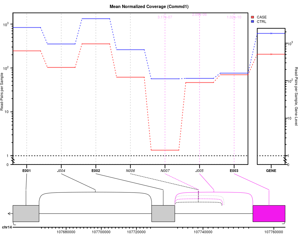
Character string. Determines which plot to produce. Options are: "expr" for "expression", or mean normalized read counts by experimental condition, "rExpr" for
"relative" expression relative to gene-level expression, "normCounts" for normalized read counts for each sample, and "rawCounts" for raw read counts for each sample.
sequencing.type
The type of sequencing used, either "paired-end" or "single-end". This only affects the labelling of the y-axis, and does not affect the actual plots in any way.
displayTranscripts
Logical. If true, then the full set of annotated transcripts will be displayed below the expression plot (to a maximum of 42 different TX).
colorList
A named list of R colors, setting the colors used for various things. See link{junctionSeqColors} for more information.
use.vst
Logical. If TRUE, all plots will be scaled via a variance stabilizing transform.
use.log
Logical. If TRUE, all plots will be log-scaled.
exon.rescale.factor
Numeric. Exons will be proportionately scaled-up so that the exonic regions make up this fraction of the horizontal plotting area. If negative, exons and introns will be plotted to a common scale.
exonRescaleFunction
Character string. Exonic and intronic regions will be rescaled to be proportional to this transformation of their span. By default the square-root function is used, which shrinks long features and extends short features so that
they are all still readable and destinguishable against one another. This default option seems to behave well on mammalian genomes. This parameter does nothing if exon.rescale.factor is negative.
label.p.vals
Logical. If TRUE, then statistically significant p-values will be labelled.
plot.lwd
the line width for the plotting lines.
axes.lwd
the line width for the axes.
anno.lwd
the line width for the various other annotation lines.
gene.lwd
the line width used for the gene annotation lines.
par.cex
The base cex value to be passed to par() immediately before all plots are created. See par.
anno.cex.text
The font size multiplier for most annotation text. This will be multiplied by a factor of the par.cex value.
More specifically: The cex value to be passed to all function calls that take graphical parameters. See par.
anno.cex.axis
The font size multiplier for the axis text. This will be multiplied by a factor of the par.cex value.
More specifically: The cex.axis value to be passed to all function calls that take graphical parameters. See par.
anno.cex.main
The font size multiplier for the main title text. This will be multiplied by a factor of the par.cex value.
More specifically: The cex.main value to be passed to all function calls that take graphical parameters. See par.
cex.arrows
The font size for the strand-direction arrows in the gene annotation region.
The arrows will be sized to equal the dimensions of the letter "M" at this font size.
fit.countbin.names
Logical. If TRUE, then splice-junction-locus labels should be rescaled to fit in whatever horizontal space is available.
fit.genomic.axis
Logical. If TRUE, then the genomic coordinate labels will be auto-scaled down to fit, if needed.
fit.labels
Logical. If TRUE, then y-axis labels will be auto-scaled down to fit, if needed. Note this only applies to the text labels, not the numeric scales.
plot.gene.level.expression
Logical value. If TRUE, gene-level expression (when applicable) will be plotted beside the sub-element-specific expression in a small seperate plotting box.
For the "relative expression" plots the simple mean normalized expression will be plotted (since it doesn't make sense to plot something relative to itself).
plot.exon.results
Logical. If TRUE, plot results for exons. By default everything that was tested will be plotted.
plot.junction.results
Logical. If TRUE, plot results for splice junctions. By default everything that was tested will be plotted.
plot.novel.junction.results
Logical. If TRUE, plot results for novel splice junctions. If false, novel splice junctions will be ignored. By default everything that was tested will be plotted.
plot.untestable.results
Logical. If TRUE, plots the expression of splice junctions that had coverage that was too low to be tested.
draw.untestable.annotation
Logical. If TRUE, draws the annotation for splice junctions that had coverage that was too low to be tested.
show.strand.arrows
The number of strand-direction arrows to display. If equal to 1 (the default) then the arrow will extend from the end of the gene drawing, if it is greater than 1 then arrows will be drawn
along the gene length. If it is 0 or NA then arrows will not be drawn.
sort.features
Logical. If TRUE, sort features by genomic position.
drawCoordinates
Whether to label the genomic coordinates at the bottom of the plot.
yAxisLabels.inExponentialForm
Logical. If TRUE, then the y-axis will be labelled in exponential form.
graph.margins
Numeric vector of length 4. These margins values used (as if for par("mar")) for the main graph. The lower part of the plot uses the same left and right margins.
GENE.annotation.relative.height
The height of the "gene track" displayed underneath the main graph, relative to the height of the main graph. By default it is 20 percent.
TX.annotation.relative.height
For all plots that draw the annotated-transcript set (when the with.TX parameter is TRUE), this sets the height of each transcript, as a fraction of the height of the main graph. By default it is 2.5 percent.
CONNECTIONS.relative.height
The height of the panel that connects the plotting area to the gene annotation area, relative to the height of the plotting area. This panel has the lines that connects the counting bin columns to their actual loci on the gene. By default it is 10 percent.
SPLICE.annotation.relative.height
The height of the area that shows the splice junction loci, relative to the size of the plotting area.
TX.margins
A numeric vector of length 2. The size of the blank space between the gene plot and the transcript list and then beneath the transcript list, relative to the size of each transcript line.
title.main
Character string. Overrides the default main plot title.
title.ylab
Character string. Overrides the default y-axis label for the left y-axis.
title.ylab.right
Character string. Overrides the default y-axis label for the right y-axis.
condition.legend.text
List or named vector of character strings. This optional parameter can be used to assign labels to each condition variable values. It should be a list or named vector with length equal to factor(condition). Each element
should be named with one of the values from factor(condition), and should contain the label. They will be listed in this order in the figure legend.
include.TX.names
Logical value. If TRUE, then for the plots that include the annotated transcript,
the transcript names will be listed. The labels will be drawn at half the size
of anno.cex.text.
draw.start.end.sites
Logical value. If TRUE, then transcript start/end sites will be marked on the main gene annotation.
label.chromosome
Logical. If TRUE, label the chromosome in the left margin.
If the text is too long it will be auto-fitted into the available margin.
splice.junction.drawing.style
The visual style of the splice junctions drawn on the gene annotation.
The default uses paired hyperbolas with the ends straightened out.
A number of other styles are available.
draw.nested.SJ
Logical. If TRUE, overlapping splice junctions will be drawn layered under one another.
This can vastly improve readability when there are a large number of overlapping splice junctions.
Default is TRUE.
merge.exon.parts
Logical. If TRUE, in the gene annotation plot merge connected exon-fragments and delineate them with dotted lines.
verbose
if TRUE, send debugging and progress messages to the console / stdout.
debug.mode
Logical. If TRUE, print additional debugging information during execution.
INTERNAL.VARS
NOT FOR GENERAL USE. Intended only for use by JunctionSeq itself, internally. This is used
for passing pre-generated data (when generating many similar plots, for example), and
for internally-generated parameters. DO NOT USE.
...
Additional options to pass to plotting functions, particularly graphical parameters.
Value
This is a side-effecting function, and does not return a value.
Examples
data(exampleDataSet,package="JctSeqData");

plotJunctionSeqResultsForGene(geneID = "ENSRNOG00000009281", jscs);


## Not run:
########################################
#Set up example data:
decoder.file <- system.file(
                  "extdata/annoFiles/decoder.bySample.txt",
                  package="JctSeqData");
decoder <- read.table(decoder.file,
                  header=TRUE,
                  stringsAsFactors=FALSE);
gff.file <- system.file(
            "extdata/cts/withNovel.forJunctionSeq.gff.gz",
            package="JctSeqData");
countFiles <- system.file(paste0("extdata/cts/",
     decoder$sample.ID,
     "/QC.spliceJunctionAndExonCounts.withNovel.forJunctionSeq.txt.gz"),
     package="JctSeqData");
######################
#Run example analysis:
jscs <- runJunctionSeqAnalyses(sample.files = countFiles,
           sample.names = decoder$sample.ID,
           condition=factor(decoder$group.ID),
           flat.gff.file = gff.file,
           analysis.type = "junctionsAndExons"
);
########################################

#Make an expression plot for a given gene:
plotJunctionSeqResultsForGene(geneID = "ENSRNOG00000009281", jscs);

#Plot normalized read counts for a given gene:
plotJunctionSeqResultsForGene(geneID = "ENSRNOG00000009281", jscs,
                    plot.type = "normCounts");

#Plot relative expression for a given gene:
plotJunctionSeqResultsForGene(geneID = "ENSRNOG00000009281", jscs,
                    plot.type = "rExpr");

#Plot raw read counts for a given gene:
plotJunctionSeqResultsForGene(geneID = "ENSRNOG00000009281", jscs,
                    plot.type = "rawCounts");

#Same thing, but with isoforms shown:
plotJunctionSeqResultsForGene(geneID = "ENSRNOG00000009281", jscs,
                    plot.type = "rawCounts",
                    displayTranscripts = TRUE);


## End(Not run)
Results
R version 3.3.1 (2016-06-21) -- "Bug in Your Hair"
Copyright (C) 2016 The R Foundation for Statistical Computing
Platform: x86_64-pc-linux-gnu (64-bit)

R is free software and comes with ABSOLUTELY NO WARRANTY.
You are welcome to redistribute it under certain conditions.
Type 'license()' or 'licence()' for distribution details.

R is a collaborative project with many contributors.
Type 'contributors()' for more information and
'citation()' on how to cite R or R packages in publications.

Type 'demo()' for some demos, 'help()' for on-line help, or
'help.start()' for an HTML browser interface to help.
Type 'q()' to quit R.

> library(JunctionSeq)
Loading required package: SummarizedExperiment
Loading required package: GenomicRanges
Loading required package: BiocGenerics
Loading required package: parallel

Attaching package: 'BiocGenerics'

The following objects are masked from 'package:parallel':

    clusterApply, clusterApplyLB, clusterCall, clusterEvalQ,
    clusterExport, clusterMap, parApply, parCapply, parLapply,
    parLapplyLB, parRapply, parSapply, parSapplyLB

The following objects are masked from 'package:stats':

    IQR, mad, xtabs

The following objects are masked from 'package:base':

    Filter, Find, Map, Position, Reduce, anyDuplicated, append,
    as.data.frame, cbind, colnames, do.call, duplicated, eval, evalq,
    get, grep, grepl, intersect, is.unsorted, lapply, lengths, mapply,
    match, mget, order, paste, pmax, pmax.int, pmin, pmin.int, rank,
    rbind, rownames, sapply, setdiff, sort, table, tapply, union,
    unique, unsplit

Loading required package: S4Vectors
Loading required package: stats4

Attaching package: 'S4Vectors'

The following objects are masked from 'package:base':

    colMeans, colSums, expand.grid, rowMeans, rowSums

Loading required package: IRanges
Loading required package: GenomeInfoDb
Loading required package: Biobase
Welcome to Bioconductor

    Vignettes contain introductory material; view with
    'browseVignettes()'. To cite Bioconductor, see
    'citation("Biobase")', and for packages 'citation("pkgname")'.

> png(filename="/home/ddbj/snapshot/RGM3/R_BC/result/JunctionSeq/plotJunctionSeqResultsForGene.Rd_%03d_medium.png", width=480, height=480)
> ### Name: plotJunctionSeqResultsForGene
> ### Title: Generate a JunctionSeq expression plot.
> ### Aliases: plotJunctionSeqResultsForGene
>
> ### ** Examples
>
> data(exampleDataSet,package="JctSeqData");
>
> plotJunctionSeqResultsForGene(geneID = "ENSRNOG00000009281", jscs);
> pJSRfG(): ENSRNOG00000009281, plot.type: expr
Starting nested heights...
>
>
> ## Not run:
> ##D ########################################
> ##D #Set up example data:
> ##D decoder.file <- system.file(
> ##D                   "extdata/annoFiles/decoder.bySample.txt",
> ##D                   package="JctSeqData");
> ##D decoder <- read.table(decoder.file,
> ##D                   header=TRUE,
> ##D                   stringsAsFactors=FALSE);
> ##D gff.file <- system.file(
> ##D             "extdata/cts/withNovel.forJunctionSeq.gff.gz",
> ##D             package="JctSeqData");
> ##D countFiles <- system.file(paste0("extdata/cts/",
> ##D      decoder$sample.ID,
> ##D      "/QC.spliceJunctionAndExonCounts.withNovel.forJunctionSeq.txt.gz"),
> ##D      package="JctSeqData");
> ##D ######################
> ##D #Run example analysis:
> ##D jscs <- runJunctionSeqAnalyses(sample.files = countFiles,
> ##D            sample.names = decoder$sample.ID,
> ##D            condition=factor(decoder$group.ID),
> ##D            flat.gff.file = gff.file,
> ##D            analysis.type = "junctionsAndExons"
> ##D );
> ##D ########################################
> ##D
> ##D #Make an expression plot for a given gene:
> ##D plotJunctionSeqResultsForGene(geneID = "ENSRNOG00000009281", jscs);
> ##D
> ##D #Plot normalized read counts for a given gene:
> ##D plotJunctionSeqResultsForGene(geneID = "ENSRNOG00000009281", jscs,
> ##D                     plot.type = "normCounts");
> ##D
> ##D #Plot relative expression for a given gene:
> ##D plotJunctionSeqResultsForGene(geneID = "ENSRNOG00000009281", jscs,
> ##D                     plot.type = "rExpr");
> ##D
> ##D #Plot raw read counts for a given gene:
> ##D plotJunctionSeqResultsForGene(geneID = "ENSRNOG00000009281", jscs,
> ##D                     plot.type = "rawCounts");
> ##D
> ##D #Same thing, but with isoforms shown:
> ##D plotJunctionSeqResultsForGene(geneID = "ENSRNOG00000009281", jscs,
> ##D                     plot.type = "rawCounts",
> ##D                     displayTranscripts = TRUE);
> ##D
> ## End(Not run)
>
>
>
>
>
> dev.off()
null device
          1
>
 .
.