R Graphical Manual

Browse All

Last data update: 2014.03.03

R: Fits the regularization paths for the kernel expectile...

KERE	R Documentation

Fits the regularization paths for the kernel expectile regression.

Description

Fits a regularization path for the kernel expectile regression at a sequence of regularization parameters lambda.

Usage

KERE(x, y, kern, lambda = NULL, eps = 1e-08, maxit = 1e4,
omega = 0.5, gamma = 1e-06, option = c("fast", "normal"))

Arguments

`x`	matrix of predictors, of dimension Np*; each row is an observation vector.
`y`	response variable.
`kern`	the built-in kernel classes in KERE. The `kern` parameter can be set to any function, of class kernel, which computes the inner product in feature space between two vector arguments. KERE provides the most popular kernel functions which can be initialized by using the following functions: `rbfdot` Radial Basis kernel function, `polydot` Polynomial kernel function, `vanilladot` Linear kernel function, `tanhdot` Hyperbolic tangent kernel function, `laplacedot` Laplacian kernel function, `besseldot` Bessel kernel function, `anovadot` ANOVA RBF kernel function, `splinedot` the Spline kernel. Objects can be created by calling the rbfdot, polydot, tanhdot, vanilladot, anovadot, besseldot, laplacedot, splinedot functions etc. (see example.)
`lambda`	a user supplied `lambda` sequence. It is better to supply a decreasing sequence of `lambda` values, if not, the program will sort user-defined `lambda` sequence in decreasing order automatically.
`eps`	convergence threshold for majorization minimization algorithm. Each majorization descent loop continues until the relative change in any coefficient \|\|alpha(new)-α(old)\|\|_2^2/\|\|α(old)\|\|_2^2 is less than `eps`. Defaults value is `1e-8`.
`maxit`	maximum number of loop iterations allowed at fixed lambda value. Default is 1e4. If models do not converge, consider increasing `maxit`.
`omega`	the parameter omega in the expectile regression model. The value must be in (0,1). Default is 0.5.
`gamma`	a scalar number. If it is specified, the number will be added to each diagonal element of the kernel matrix as perturbation. The default is `1e-06`.
`option`	users can choose which method to use to update the inverse matrix in the MM algorithm. `"fast"` uses a trick described in Yang, Zhang and Zou (2015) to update estimates for each lambda. `"normal"` uses a naive way for the computation.

Details

Note that the objective function in KERE is

Loss(y- α_0 - K * α )) + λ * α^T * K * α,

where the α_0 is the intercept, α is the solution vector, and K is the kernel matrix with K_{ij}=K(x_i,x_j). Users can specify the kernel function to use, options include Radial Basis kernel, Polynomial kernel, Linear kernel, Hyperbolic tangent kernel, Laplacian kernel, Bessel kernel, ANOVA RBF kernel, the Spline kernel. Users can also tweak the penalty by choosing different lambda.

For computing speed reason, if models are not converging or running slow, consider increasing eps before increasing maxit.

Value

An object with S3 class KERE.

`call`	the call that produced this object.
`alpha`	a `nrow(x)*length(lambda)` matrix of coefficients. Each column is a solution vector corresponding to a lambda value in the lambda sequence.
`lambda`	the actual sequence of `lambda` values used.
`npass`	total number of loop iterations corresponding to each lambda value.
`jerr`	error flag, for warnings and errors, 0 if no error.

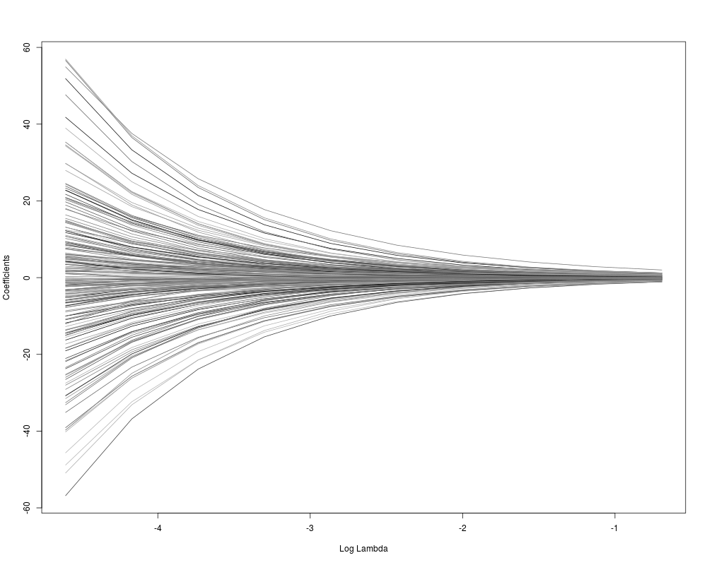
Author(s)

Yi Yang, Teng Zhang and Hui Zou
Maintainer: Yi Yang <yiyang@umn.edu>

References

Y. Yang, T. Zhang, and H. Zou. "Flexible Expectile Regression in Reproducing Kernel Hilbert Space." ArXiv e-prints: stat.ME/1508.05987, August 2015.

Examples

# create data
N <- 200
X1 <- runif(N)
X2 <- 2*runif(N)
X3 <- 3*runif(N)
SNR <- 10 # signal-to-noise ratio
Y <- X1**1.5 + 2 * (X2**.5) + X1*X3
sigma <- sqrt(var(Y)/SNR)
Y <- Y + X2*rnorm(N,0,sigma)
X <- cbind(X1,X2,X3)

# set gaussian kernel 
kern <- rbfdot(sigma=0.1)

# define lambda sequence
lambda <- exp(seq(log(0.5),log(0.01),len=10))

# run KERE
m1 <- KERE(x=X, y=Y, kern=kern, lambda = lambda, omega = 0.5) 

# plot the solution paths
plot(m1)

Results


R version 3.3.1 (2016-06-21) -- "Bug in Your Hair"
Copyright (C) 2016 The R Foundation for Statistical Computing
Platform: x86_64-pc-linux-gnu (64-bit)

R is free software and comes with ABSOLUTELY NO WARRANTY.
You are welcome to redistribute it under certain conditions.
Type 'license()' or 'licence()' for distribution details.

R is a collaborative project with many contributors.
Type 'contributors()' for more information and
'citation()' on how to cite R or R packages in publications.

Type 'demo()' for some demos, 'help()' for on-line help, or
'help.start()' for an HTML browser interface to help.
Type 'q()' to quit R.

> library(KERE)
> png(filename="/home/ddbj/snapshot/RGM3/R_CC/result/KERE/KERE.Rd_%03d_medium.png", width=480, height=480)
> ### Name: KERE
> ### Title: Fits the regularization paths for the kernel expectile
> ###   regression.
> ### Aliases: KERE
> ### Keywords: models regression
> 
> ### ** Examples
> 
> # create data
> N <- 200
> X1 <- runif(N)
> X2 <- 2*runif(N)
> X3 <- 3*runif(N)
> SNR <- 10 # signal-to-noise ratio
> Y <- X1**1.5 + 2 * (X2**.5) + X1*X3
> sigma <- sqrt(var(Y)/SNR)
> Y <- Y + X2*rnorm(N,0,sigma)
> X <- cbind(X1,X2,X3)
> 
> # set gaussian kernel 
> kern <- rbfdot(sigma=0.1)
> 
> # define lambda sequence
> lambda <- exp(seq(log(0.5),log(0.01),len=10))
> 
> # run KERE
> m1 <- KERE(x=X, y=Y, kern=kern, lambda = lambda, omega = 0.5) 
> 
> # plot the solution paths
> plot(m1)
> 
> 
> 
> 
> 
> 
> dev.off()
null device 
          1 
>