R Graphical Manual

Browse All

Last data update: 2014.03.03

R: KFAS: Functions for Exponential Family State Space Models

KFAS	R Documentation

KFAS: Functions for Exponential Family State Space Models

Description

Package KFAS contains functions for Kalman filtering, smoothing and simulation of linear state space models with exact diffuse initialization.

Details

Note, this help page might be more readable in pdf format due to the mathematical formulas containing subscripts.

The linear Gaussian state space model is given by

y[t] = Z[t]α[t] + ε[t], (observation equation)

α[t+1] = T[t]α[t] + R[t]η[t], (transition equation)

where ε[t] ~ N(0, H[t]), η[t] ~ N(0, Q[t]) and α[1] ~ N(a[1], P[1]) independently of each other.

All system and covariance matrices Z, H, T, R and Q can be time-varying, and partially or totally missing observations y[t] are allowed.

Covariance matrices H and Q has to be positive semidefinite (although this is not checked).

Model components in KFAS are defined as

y: A n x p matrix containing the observations.
Z: A p x m x 1 or p x m x n array corresponding to the system matrix of observation equation.
H: A p x p x 1 or p x p x n array corresponding to the covariance matrix of observational disturbances epsilon.
T: A m x m x 1 or m x m x n array corresponding to the first system matrix of state equation.
R: A m x k x 1 or m x k x n array corresponding to the second system matrix of state equation.
Q: A k x k x 1 or k x k x n array corresponding to the covariance matrix of state disturbances eta
a1: A m x 1 matrix containing the expected values of the initial states.
P1: A m x m matrix containing the covariance matrix of the nondiffuse part of the initial state vector.
P1inf: A m x m matrix containing the covariance matrix of the diffuse part of the initial state vector.
u: A n x p matrix of an additional parameters in case of non-Gaussian model.

In case of any of the series in model is defined as non-Gaussian, the observation equation is of form

∏[i]^p p(y[t, i]|θ[t]),

with θ[t, i] = Z[i, t]α[t] being one of the following:

y[t]~N(μ[t], u[t]), with identity link θ[t] = μ[t]. Note that now variances are defined using u_t, not H_t. If the correlation between Gaussian observation equations is needed, one can use u[t] = 0 and add correlating disturbances into state equation (although care is then needed when making inferences about signal which contains the error terms also).
y[t]~Poisson(u[t]λ[t]), where u[t] is an offset term, with θ[t] = log(u[t]λ[t]).
y[t]~binomial(u[t], π[t]), with θ[t] = log(π[t]/(1-π[t])), where π[t] is the probability of success at time t.
y[t]~gamma(u[t], μ[t]), with [θ[t] = log(μ[t])], where μ[t] is the mean parameter and u[t] is the shape parameter.
y[t]~negative binomial(u[t], μ[t]), with expected value μ[t] and variance μ[t]+ μ[t]^2/u[t] (see dnbinom), then θ[t] = log(μ[t]).

For exponential family models u[t] = 1 as a default. For completely Gaussian models, parameter is omitted. Note that series can have different distributions in case of multivariate models.

For the unknown elements of initial state vector a[1], KFAS uses exact diffuse initialization by Koopman and Durbin (2000, 2012, 2003), where the unknown initial states are set to have a zero mean and infinite variance, so

P[1] = P[*, 1] + κP[inf, 1],

with κ going to infinity and P[inf, 1] being diagonal matrix with ones on diagonal elements corresponding to unknown initial states.

This method is basically a equivalent of setting uninformative priors for the initial states in a Bayesian framework.

Diffuse phase is continued until rank of P[inf, t] becomes zero. Rank of P[inf, t] decreases by 1, if F[inf, t]>ξ[t]>0, where ξ[t] is by default .Machine$double.eps^0.5*max(Z[, , t]^2). Usually the number of diffuse time points equals the number unknown elements of initial state vector, but missing observations or time-varying system matrices can affect this. See Koopman and Durbin (2000, 2012, 2003) for details for exact diffuse and non-diffuse filtering. If the number of diffuse states is large compared to the data, it is possible that the model is degenerate in a sense that not enough information is available for leaving the diffuse phase.

To lessen the notation and storage space, KFAS uses letters P, F and K for non-diffuse part of the corresponding matrices, omitting the asterisk in diffuse phase.

All functions of KFAS use the univariate approach (also known as sequential processing, see Anderson and Moore (1979)) which is from Koopman and Durbin (2000, 2012). In univariate approach the observations are introduced one element at the time. Therefore the prediction error variance matrices F and Finf do not need to be non-singular, as there is no matrix inversions in univariate approach algorithm. This provides possibly more faster filtering and smoothing than normal multivariate Kalman filter algorithm, and simplifies the formulas for diffuse filtering and smoothing. If covariance matrix H is not diagonal, it is possible to transform the model by either using LDL decomposition on H, or augmenting the state vector with ε disturbances (this is done automatically in KFAS if needed). See transformSSM for more details.

References

Koopman, S.J. and Durbin J. (2000). Fast filtering and smoothing for non-stationary time series models, Journal of American Statistical Assosiation, 92, 1630-38.

Koopman, S.J. and Durbin J. (2012). Time Series Analysis by State Space Methods. Second edition. Oxford: Oxford University Press.

Koopman, S.J. and Durbin J. (2003). Filtering and smoothing of state vector for diffuse state space models, Journal of Time Series Analysis, Vol. 24, No. 1.

Shumway, Robert H. and Stoffer, David S. (2006). Time Series Analysis and Its Applications: With R examples.

Examples


# Example of local level model for Nile series
# See Durbin and Koopman (2012)

model_Nile <- SSModel(Nile ~
  SSMtrend(1, Q = list(matrix(NA))), H = matrix(NA))
model_Nile
model_Nile <- fitSSM(model_Nile, c(log(var(Nile)), log(var(Nile))),
  method = "BFGS")$model

# Filtering and state smoothing
out_Nile <- KFS(model_Nile, filtering = "state", smoothing = "state")
out_Nile

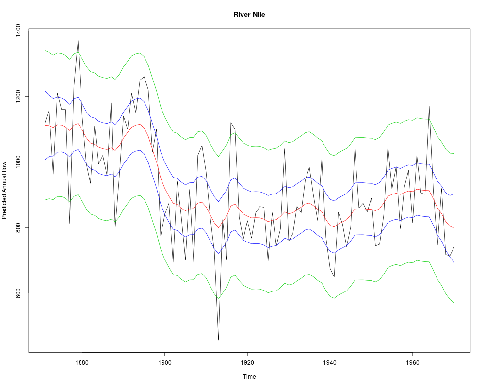
# Confidence and prediction intervals for the expected value and the observations.
# Note that predict uses original model object, not the output from KFS.
conf_Nile <- predict(model_Nile, interval = "confidence", level = 0.9)
pred_Nile <- predict(model_Nile, interval = "prediction", level = 0.9)

ts.plot(cbind(Nile, pred_Nile, conf_Nile[, -1]), col = c(1:2, 3, 3, 4, 4),
        ylab = "Predicted Annual flow", main = "River Nile")


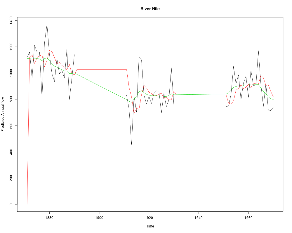
# Missing observations, using the same parameter estimates

NileNA <- Nile
NileNA[c(21:40, 61:80)] <- NA
model_NileNA <- SSModel(NileNA ~ SSMtrend(1, Q = list(model_Nile$Q)),
H = model_Nile$H)

out_NileNA <- KFS(model_NileNA, "mean", "mean")

# Filtered and smoothed states
ts.plot(NileNA, fitted(out_NileNA, filtered = TRUE), fitted(out_NileNA),
  col = 1:3, ylab = "Predicted Annual flow",
  main = "River Nile")


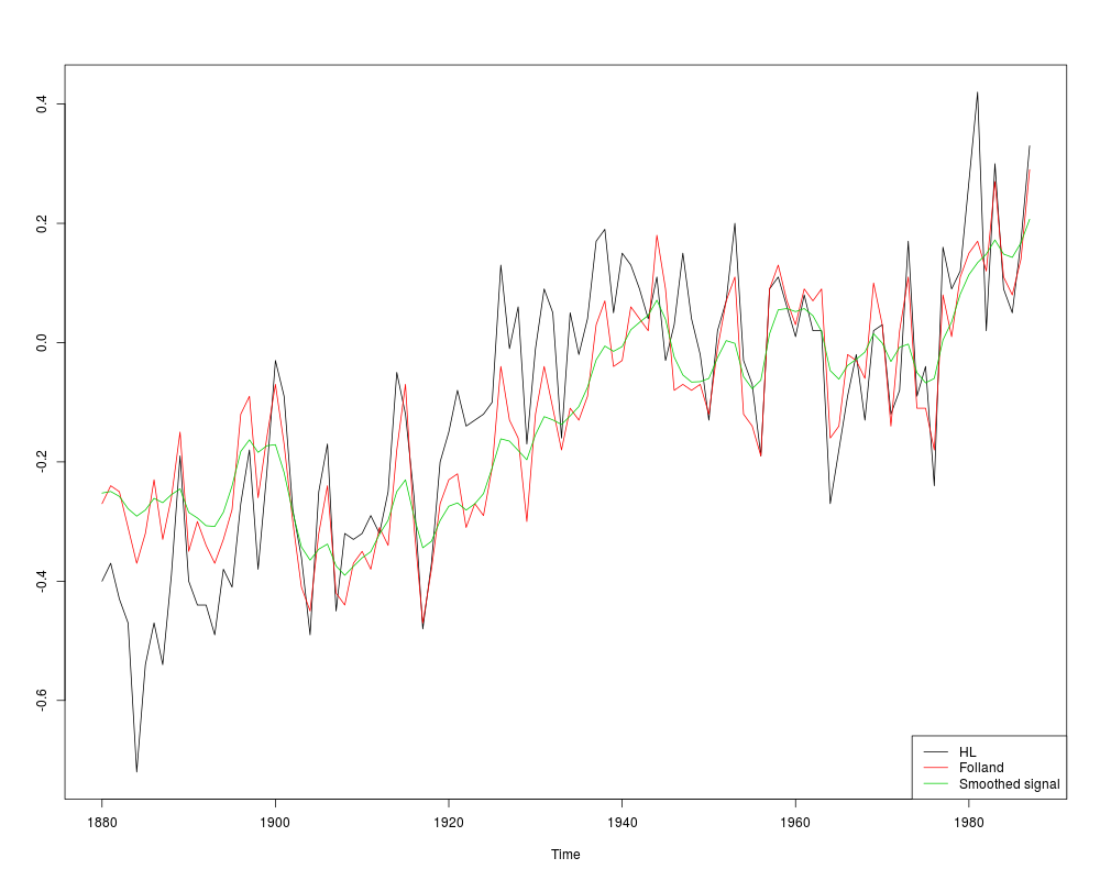
# Example of multivariate local level model with only one state
# Two series of average global temperature deviations for years 1880-1987
# See Shumway and Stoffer (2006), p. 327 for details

data("GlobalTemp")

model_temp <- SSModel(GlobalTemp ~ SSMtrend(1, Q = NA, type = "common"),
  H = matrix(NA, 2, 2))

# Estimating the variance parameters
inits <- chol(cov(GlobalTemp))[c(1, 4, 3)]
inits[1:2] <- log(inits[1:2])
fit_temp <- fitSSM(model_temp, c(0.5*log(.1), inits), method = "BFGS")

out_temp <- KFS(fit_temp$model)

ts.plot(cbind(model_temp$y, coef(out_temp)), col = 1:3)
legend("bottomright",
  legend = c(colnames(GlobalTemp), "Smoothed signal"), col = 1:3, lty = 1)


## Not run: 
# Seatbelts data
# See Durbin and Koopman (2012)

model_drivers <- SSModel(log(drivers) ~ SSMtrend(1, Q = list(NA))+
   SSMseasonal(period = 12, sea.type = "trigonometric", Q = NA) +
   log(PetrolPrice) + law, data = Seatbelts, H = NA)

# As trigonometric seasonal contains several disturbances which are all
# identically distributed, default behaviour of fitSSM is not enough,
# as we have constrained Q. We can either provide our own
# model updating function with fitSSM, or just use optim directly:

# option 1:
ownupdatefn <- function(pars, model){
  model$H[] <- exp(pars[1])
  diag(model$Q[, , 1]) <- exp(c(pars[2], rep(pars[3], 11)))
  model #for optim, replace this with -logLik(model) and call optim directly
}

fit_drivers <- fitSSM(model_drivers,
  log(c(var(log(Seatbelts[, "drivers"])), 0.001, 0.0001)),
  ownupdatefn, method = "BFGS")

out_drivers <- KFS(fit_drivers$model, smoothing = c("state", "mean"))
out_drivers
ts.plot(out_drivers$model$y, fitted(out_drivers), lty = 1:2, col = 1:2,
  main = "Observations and smoothed signal with and without seasonal component")
lines(signal(out_drivers, states = c("regression", "trend"))$signal,
  col = 4, lty = 1)
legend("bottomleft", col = c(1, 2, 4), lty = c(1, 2, 1),
  legend = c("Observations", "Smoothed signal", "Smoothed level"))

# Multivariate model with constant seasonal pattern,
# using the the seat belt law dummy only for the front seat passangers,
# and restricting the rank of the level component by using custom component

model_drivers2 <- SSModel(log(cbind(front, rear)) ~ -1 +
    log(PetrolPrice) + log(kms) +
    SSMregression(~law, data = Seatbelts, index = 1) +
    SSMcustom(Z = diag(2), T = diag(2), R = matrix(1, 2, 1),
      Q = matrix(1), P1inf = diag(2)) +
    SSMseasonal(period = 12, sea.type = "trigonometric"),
  data = Seatbelts, H = matrix(NA, 2, 2))

# An alternative way for defining the rank deficient trend component:

# model_drivers2 <- SSModel(log(cbind(front, rear)) ~ -1 +
#     log(PetrolPrice) + log(kms) +
#     SSMregression(~law, data = Seatbelts, index = 1) +
#     SSMtrend(degree = 1, Q = list(matrix(0, 2, 2))) +
#     SSMseasonal(period = 12, sea.type = "trigonometric"),
#   data = Seatbelts, H = matrix(NA, 2, 2))
#
# Modify model manually:
# model_drivers2$Q <- array(1, c(1, 1, 1))
# model_drivers2$R <- model_drivers2$R[, -2, , drop = FALSE]
# attr(model_drivers2, "k") <- 1L
# attr(model_drivers2, "eta_types") <- attr(model_drivers2, "eta_types")[1]


likfn <- function(pars, model, estimate = TRUE){
  diag(model$H[, , 1]) <- exp(0.5 * pars[1:2])
  model$H[1, 2, 1] <- model$H[2, 1, 1] <-
    tanh(pars[3]) * prod(sqrt(exp(0.5 * pars[1:2])))
  model$R[28:29] <- exp(pars[4:5])
  if(estimate) return(-logLik(model))
  model
}

fit_drivers2 <- optim(f = likfn, p = c(-8, -8, 1, -1, -3), method = "BFGS",
  model = model_drivers2)
model_drivers2 <- likfn(fit_drivers2$p, model_drivers2, estimate = FALSE)
model_drivers2$R[28:29, , 1]%*%t(model_drivers2$R[28:29, , 1])
model_drivers2$H

out_drivers2 <- KFS(model_drivers2)
out_drivers2
ts.plot(signal(out_drivers2, states = c("custom", "regression"))$signal,
  model_drivers2$y, col = 1:4)

# For confidence or prediction intervals, use predict on the original model
pred <- predict(model_drivers2,
  states = c("custom", "regression"), interval = "prediction")

# Note that even though the intervals were computed without seasonal pattern,
# PetrolPrice induces seasonal pattern to predictions
ts.plot(pred$front, pred$rear, model_drivers2$y,
  col = c(1, 2, 2, 3, 4, 4, 5, 6), lty = c(1, 2, 2, 1, 2, 2, 1, 1))

## End(Not run)

## Simulate ARMA(2, 2) process
set.seed(1)
y <- arima.sim(n = 1000, list(ar = c(0.8897, -0.4858), ma = c(-0.2279, 0.2488)),
               innov = rnorm(1000) * sqrt(0.5))


model_arima <- SSModel(y ~ SSMarima(ar = c(0, 0), ma = c(0, 0), Q = 1), H = 0)

likfn <- function(pars, model, estimate = TRUE){
  tmp <- try(SSMarima(artransform(pars[1:2]), artransform(pars[3:4]),
    Q = exp(pars[5])), silent = TRUE)
  if(!inherits(tmp, "try-error")){
    model["T", "arima"] <- tmp$T
    model["R", "arima"] <- tmp$R
    model["P1", "arima"] <- tmp$P1
    model["Q", "arima"] <- tmp$Q
    if(estimate){
      -logLik(model)
    } else model
  } else {
    if(estimate){
      1e100
    } else model
  }
}

fit_arima <- optim(par = c(rep(0, 4), log(1)), fn = likfn, method = "BFGS",
  model = model_arima)
model_arima <- likfn(fit_arima$par, model_arima, FALSE)

# AR coefficients:
model_arima$T[2:3, 2, 1]
# MA coefficients:
model_arima$R[3:4]
# sigma2:
model_arima$Q[1]
# intercept
KFS(model_arima)
# same with arima:
arima(y, c(2, 0, 2))
# small differences because the intercept is handled differently in arima

## Not run: 
# Poisson model
# See Durbin and Koopman (2012)
model_van <- SSModel(VanKilled ~ law + SSMtrend(1, Q = list(matrix(NA)))+
               SSMseasonal(period = 12, sea.type = "dummy", Q = NA),
               data = Seatbelts, distribution = "poisson")

# Estimate variance parameters
fit_van <- fitSSM(model_van, c(-4, -7), method = "BFGS")

model_van <- fit_van$model

# use approximating model, gives posterior modes
out_nosim <- KFS(model_van, nsim = 0)
# State smoothing via importance sampling
out_sim <- KFS(model_van, nsim = 1000)

out_nosim
out_sim

## End(Not run)

##########################################################
### Examples of generalized linear modelling with KFAS ###
##########################################################

# Same example as in ?glm
counts <- c(18, 17, 15, 20, 10, 20, 25, 13, 12)
outcome <- gl(3, 1, 9)
treatment <- gl(3, 3)
glm_D93 <- glm(counts ~ outcome + treatment, family = poisson())

model_D93 <- SSModel(counts ~ outcome + treatment,
  distribution = "poisson")

out_D93 <- KFS(model_D93)
coef(out_D93, last = TRUE)
coef(glm_D93)

summary(glm_D93)$cov.s
out_D93$V[, , 1]

# approximating model as in GLM
out_D93_nosim <- KFS(model_D93, smoothing = c("state", "signal", "mean"))

# with importance sampling. Number of simulations is too small here,
# with large enough nsim the importance sampling actually gives
# very similar results as the approximating model in this case
set.seed(1)
out_D93_sim <- KFS(model_D93,
  smoothing = c("state", "signal", "mean"), nsim = 1000)


## linear predictor
# GLM
glm_D93$linear.predictor
# approximate model, this is the posterior mode of p(theta|y)
c(out_D93_nosim$thetahat)
# importance sampling on theta, gives E(theta|y)
c(out_D93_sim$thetahat)


## predictions on response scale
# GLM
fitted(glm_D93)
# approximate model with backtransform, equals GLM
fitted(out_D93_nosim)
# importance sampling on exp(theta)
fitted(out_D93_sim)

# prediction variances on link scale
# GLM
as.numeric(predict(glm_D93, type = "link", se.fit = TRUE)$se.fit^2)
# approx, equals to GLM results
c(out_D93_nosim$V_theta)
# importance sampling on theta
c(out_D93_sim$V_theta)


# prediction variances on response scale
# GLM
as.numeric(predict(glm_D93, type = "response", se.fit = TRUE)$se.fit^2)
# approx, equals to GLM results
c(out_D93_nosim$V_mu)
# importance sampling on theta
c(out_D93_sim$V_mu)

# A Gamma example modified from ?glm
# Now with log-link, and identical intercept terms
clotting <- data.frame(
u = c(5,10,15,20,30,40,60,80,100),
lot1 = c(118,58,42,35,27,25,21,19,18),
lot2 = c(69,35,26,21,18,16,13,12,12))

model_gamma <- SSModel(cbind(lot1, lot2) ~ -1 + log(u) +
    SSMregression(~ 1, type = "common", remove.intercept = FALSE),
  data = clotting, distribution = "gamma")

update_shapes <- function(pars, model) {
  model$u[, 1] <- pars[1]
  model$u[, 2] <- pars[2]
  model
}
fit_gamma <- fitSSM(model_gamma, inits = c(1, 1), updatefn = update_shapes,
method = "L-BFGS-B", lower = 0, upper = 100)
logLik(fit_gamma$model)
KFS(fit_gamma$model)
fit_gamma$model["u", times = 1]



## Not run: 
####################################
### Linear mixed model with KFAS ###
####################################

# example from ?lmer of lme4 pacakge
data("sleepstudy", package = "lme4")

model_lmm <- SSModel(Reaction ~ Days +
    SSMregression(~ Days, Q = array(0, c(2, 2, 180)),
       P1 = matrix(NA, 2, 2), remove.intercept = FALSE), sleepstudy, H = NA)

# The first 10 time points the third and fouth state
# defined with SSMregression correspond to the first subject, and next 10 time points
# are related to second subject and so on.

# need to use ordinary $ assignment as [ assignment operator for SSModel
# object guards against dimension altering
model_lmm$T <- array(model_lmm["T"], c(4, 4, 180))
attr(model_lmm, "tv")[3] <- 1L #needs to be integer type!

# "cut the connection" between the subjects
times <- seq(10, 180, by = 10)
model_lmm["T",states = 3:4, times = times] <- 0

# for the first subject the variance of the random effect is defined via P1
# for others, we use Q
model_lmm["Q", times = times] <- NA

update_lmm <- function(pars = init, model){
  P1 <- diag(exp(pars[1:2]))
  P1[1, 2] <- pars[3]
  model["P1", states = 3:4] <- model["Q", times = times] <-
    crossprod(P1)
  model["H"] <- exp(pars[4])
  model
}

inits <- c(0, 0, 0, 3)

fit_lmm <- fitSSM(model_lmm, inits, update_lmm, method = "BFGS")
out_lmm <- KFS(fit_lmm$model)
# unconditional covariance matrix of random effects
fit_lmm$model["P1", states = 3:4]

# conditional covariance matrix of random effects
# same for each subject and time point due to model structure
# these differ from the ones obtained from lmer as these are not conditioned
# on the fixed effects
out_lmm$V[3:4,3:4,1]

## End(Not run)
## Not run: 
# Example of Cubic spline smoothing
# See Durbin and Koopman (2012)
require("MASS")
data("mcycle")

model <- SSModel(accel ~ -1 +
    SSMcustom(Z = matrix(c(1, 0), 1, 2),
      T = array(diag(2), c(2, 2, nrow(mcycle))),
      Q = array(0, c(2, 2, nrow(mcycle))),
      P1inf = diag(2), P1 = diag(0, 2)), data = mcycle)

model$T[1, 2, ] <- c(diff(mcycle$times), 1)
model$Q[1, 1, ] <- c(diff(mcycle$times), 1)^3/3
model$Q[1, 2, ] <- model$Q[2, 1, ] <- c(diff(mcycle$times), 1)^2/2
model$Q[2, 2, ] <- c(diff(mcycle$times), 1)


updatefn <- function(pars, model, ...){
  model["H"] <- exp(pars[1])
  model["Q"] <- model["Q"] * exp(pars[2])
  model
}

fit <- fitSSM(model, inits = c(4, 4), updatefn = updatefn, method = "BFGS")

pred <- predict(fit$model, interval = "conf", level = 0.95)
plot(x = mcycle$times, y = mcycle$accel, pch = 19)
lines(x = mcycle$times, y = pred[, 1])
lines(x = mcycle$times, y = pred[, 2], lty = 2)
lines(x = mcycle$times, y = pred[, 3], lty = 2)

## End(Not run)

Results