R Graphical Manual

Browse All

Last data update: 2014.03.03

R: State Space Model Predictions

predict.SSModel

R Documentation

State Space Model Predictions

Description

Function predict.SSModel predicts the future observations of a state space model of class SSModel.

Usage

## S3 method for class 'SSModel'
predict(object, newdata, n.ahead, interval = c("none",
  "confidence", "prediction"), level = 0.95, type = c("response", "link"),
  states = NULL, se.fit = FALSE, nsim = 0, prob = TRUE, maxiter = 50,
  filtered = FALSE, ...)

Arguments

`object`	Object of class `SSModel`.
`newdata`	A compatible `SSModel` object to be added in the end of the old object for which the predictions are required. If omitted, predictions are either for the past data points, or if argument `n.ahead` is given, `n.ahead` time steps ahead.
`n.ahead`	Number of steps ahead at which to predict. Only used if `newdata` is omitted. Note that when using `n.ahead`, object cannot contain time varying system matrices.
`interval`	Type of interval calculation.
`level`	Confidence level for intervals.
`type`	Scale of the prediction, `"response"` or `"link"`.
`states`	Which states are used in computing the predictions. Either a numeric vector containing the indices of the corresponding states, or a character vector defining the types of the corresponding states. Possible choices are `"all"`, `"level"`, `"slope"`, `"trend"`, `"regression"`, `"arima"`, `"custom"`, `"cycle"` or `"seasonal"`, where `"trend"` extracts all states relating to trend. These can be combined. Default is `"all"`.
`se.fit`	If TRUE, standard errors of fitted values are computed. Default is FALSE.
`nsim`	Number of independent samples used in importance sampling. Used only for non-Gaussian models.
`prob`	if TRUE (default), the predictions in binomial case are probabilities instead of counts.
`maxiter`	The maximum number of iterations used in approximation Default is 50. Only used for non-Gaussian model.
`filtered`	If `TRUE`, compute predictions based on filtered (one-step-ahead) estimates. Default is FALSE i.e. predictions are based on all available observations given by user. For diffuse phase, interval bounds and standard errors of fitted values are set to `-Inf`/`Inf` (If the interest is in the first time points it might be useful to use non-exact diffuse initialization.).
`...`	Ignored.

Details

For non-Gaussian models, the results depend whether importance sampling is used (nsim>0). without simulations, the confidence intervals are based on the Gaussian approximation of p(α | y). Confidence intervals in response scale are computed in linear predictor scale, and then transformed to response scale. The prediction intervals are not supported. 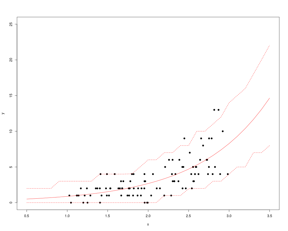With importance sampling, the confidence intervals are computed as the empirical quantiles from the weighted sample, whereas the prediction intervals contain additional step of simulating the response variables from the sampling distribution p(y|θ^i).

Predictions take account the uncertainty in state estimation (given the prior distribution for the initial states), but not the uncertainty of estimating the parameters in the system matrices (i.e. Z, Q etc.). Thus the obtained confidence/prediction intervals can underestimate the true uncertainty for short time series and/or complex models.

If no simulations are used, the standard errors in response scale are computed using the Delta method.

Value

A matrix or list of matrices containing the predictions, and optionally standard errors.

Examples


set.seed(1)
x <- runif(n=100,min=1,max=3)
y <- rpois(n=100,lambda=exp(x-1))
model <- SSModel(y~x,distribution="poisson")
xnew <- seq(0.5,3.5,by=0.1)
newdata <- SSModel(rep(NA,length(xnew))~xnew,distribution="poisson")
pred <- predict(model,newdata=newdata,interval="prediction",level=0.9,nsim=100)
plot(x=x,y=y,pch=19,ylim=c(0,25),xlim=c(0.5,3.5))
matlines(x=xnew,y=pred,col=c(2,2,2),lty=c(1,2,2),type="l")

model <- SSModel(Nile~SSMtrend(1,Q=1469),H=15099)
pred <- predict(model,n.ahead=10,interval="prediction",level=0.9)
pred

Results


R version 3.3.1 (2016-06-21) -- "Bug in Your Hair"
Copyright (C) 2016 The R Foundation for Statistical Computing
Platform: x86_64-pc-linux-gnu (64-bit)

R is free software and comes with ABSOLUTELY NO WARRANTY.
You are welcome to redistribute it under certain conditions.
Type 'license()' or 'licence()' for distribution details.

R is a collaborative project with many contributors.
Type 'contributors()' for more information and
'citation()' on how to cite R or R packages in publications.

Type 'demo()' for some demos, 'help()' for on-line help, or
'help.start()' for an HTML browser interface to help.
Type 'q()' to quit R.

> library(KFAS)
> png(filename="/home/ddbj/snapshot/RGM3/R_CC/result/KFAS/predict.SSModel.Rd_%03d_medium.png", width=480, height=480)
> ### Name: predict.SSModel
> ### Title: State Space Model Predictions
> ### Aliases: predict predict.SSModel
> 
> ### ** Examples
> 
> 
> set.seed(1)
> x <- runif(n=100,min=1,max=3)
> y <- rpois(n=100,lambda=exp(x-1))
> model <- SSModel(y~x,distribution="poisson")
> xnew <- seq(0.5,3.5,by=0.1)
> newdata <- SSModel(rep(NA,length(xnew))~xnew,distribution="poisson")
> pred <- predict(model,newdata=newdata,interval="prediction",level=0.9,nsim=100)
> plot(x=x,y=y,pch=19,ylim=c(0,25),xlim=c(0.5,3.5))
> matlines(x=xnew,y=pred,col=c(2,2,2),lty=c(1,2,2),type="l")
> 
> model <- SSModel(Nile~SSMtrend(1,Q=1469),H=15099)
> pred <- predict(model,n.ahead=10,interval="prediction",level=0.9)
> pred
Time Series:
Start = 1971 
End = 1980 
Frequency = 1 
          fit      lwr      upr
1971 798.3727 562.2916 1034.454
1972 798.3727 554.0190 1042.726
1973 798.3727 546.0174 1050.728
1974 798.3727 538.2619 1058.484
1975 798.3727 530.7310 1066.014
1976 798.3727 523.4063 1073.339
1977 798.3727 516.2717 1080.474
1978 798.3727 509.3132 1087.432
1979 798.3727 502.5183 1094.227
1980 798.3727 495.8760 1100.870
> 
> 
> 
> 
> 
> dev.off()
null device 
          1 
>