Supported by Dr. Osamu Ogasawara and  . . |
|
Last data update: 2014.03.03 |
Simulation of a Gaussian State Space ModelDescriptionFunction Usage
simulateSSM(object, type = c("states", "signals", "disturbances",
  "observations", "epsilon", "eta"), filtered = FALSE, nsim = 1,
  antithetics = FALSE, conditional = TRUE)
Arguments
DetailsSimulation smoother algorithm is based on article by J. Durbin and S.J. Koopman (2002).
The simulation filter ( Function can use two antithetic variables, one for location and other for scale, so output contains four blocks of simulated values which correlate which each other (ith block correlates negatively with (i+1)th block, and positively with (i+2)th block etc.). Note that KFAS versions 1.2.0 and older, for unconditional simulation the initial
distribution of states was fixed so that ValueAn n x k x nsim array containing the simulated series, where k is number of observations, signals, states or disturbances. ReferencesDurbin J. and Koopman, S.J. (2002). A simple and efficient simulation smoother for state space time series analysis, Biometrika, Volume 89, Issue 3 Examplesset.seed(123) # simulate new observations from the "fitted" model model <- SSModel(Nile ~ SSMtrend(1, Q = 1469), H = 15099) # signal conditional on the data i.e. samples from p(theta | y) # unconditional simulation is not reasonable as the model is nonstationary signal_sim <- simulateSSM(model, type = "signals", nsim = 10) # and add unconditional noise term i.e samples from p(epsilon) epsilon_sim <- simulateSSM(model, type = "epsilon", nsim = 10, conditional = FALSE) observation_sim <- signal_sim + epsilon_sim ts.plot(observation_sim[,1,], Nile, col = c(rep(2, 10), 1), lty = c(rep(2, 10), 1), lwd = c(rep(1, 10), 2)) # fully unconditional simulation: observation_sim2 <- simulateSSM(model, type = "observations", nsim = 10, conditional = FALSE) ts.plot(observation_sim[,1,], observation_sim2[,1,], Nile, col = c(rep(2:3, each = 10), 1), lty = c(rep(2, 20), 1), lwd = c(rep(1, 20), 2)) # illustrating use of antithetics model <- SSModel(matrix(NA, 100, 1) ~ SSMtrend(1, 1, P1inf = 0), H = 1) set.seed(123) sim <- simulateSSM(model, "obs", nsim = 2, antithetics = TRUE) # first time points sim[1,,] # correlation structure between simulations with two antithetics cor(sim[,1,]) out_NA <- KFS(model, filtering = "none", smoothing = "state") model["y"] <- sim[, 1, 1] out_obs <- KFS(model, filtering = "none", smoothing = "state") set.seed(40216) # simulate states from the p(alpha | y) sim_conditional <- simulateSSM(model, nsim = 10, antithetics = TRUE) # mean of the simulated states is exactly correct due to antithetic variables mean(sim_conditional[2, 1, ]) out_obs$alpha[2] # for variances more simulations are needed var(sim_conditional[2, 1, ]) out_obs$V[2] set.seed(40216) # no data, simulations from p(alpha) sim_unconditional <- simulateSSM(model, nsim = 10, antithetics = TRUE, conditional = FALSE) mean(sim_unconditional[2, 1, ]) out_NA$alpha[2] var(sim_unconditional[2, 1, ]) out_NA$V[2] ts.plot(cbind(sim_conditional[,1,1:5], sim_unconditional[,1,1:5]), col = rep(c(2,4), each = 5)) lines(out_obs$alpha, lwd=2) Results
R version 3.3.1 (2016-06-21) -- "Bug in Your Hair"
Copyright (C) 2016 The R Foundation for Statistical Computing
Platform: x86_64-pc-linux-gnu (64-bit)
R is free software and comes with ABSOLUTELY NO WARRANTY.
You are welcome to redistribute it under certain conditions.
Type 'license()' or 'licence()' for distribution details.
R is a collaborative project with many contributors.
Type 'contributors()' for more information and
'citation()' on how to cite R or R packages in publications.
Type 'demo()' for some demos, 'help()' for on-line help, or
'help.start()' for an HTML browser interface to help.
Type 'q()' to quit R.
> library(KFAS)
> png(filename="/home/ddbj/snapshot/RGM3/R_CC/result/KFAS/simulateSSM.Rd_%03d_medium.png", width=480, height=480)
> ### Name: simulateSSM
> ### Title: Simulation of a Gaussian State Space Model
> ### Aliases: simulateSSM
>
> ### ** Examples
>
>
> set.seed(123)
> # simulate new observations from the "fitted" model
> model <- SSModel(Nile ~ SSMtrend(1, Q = 1469), H = 15099)
> # signal conditional on the data i.e. samples from p(theta | y)
> # unconditional simulation is not reasonable as the model is nonstationary
> signal_sim <- simulateSSM(model, type = "signals", nsim = 10)
> # and add unconditional noise term i.e samples from p(epsilon)
> epsilon_sim <- simulateSSM(model, type = "epsilon", nsim = 10,
+ conditional = FALSE)
> observation_sim <- signal_sim + epsilon_sim
>
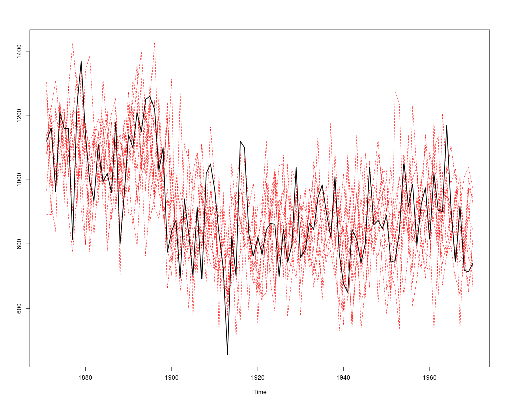
> ts.plot(observation_sim[,1,], Nile, col = c(rep(2, 10), 1),
+ lty = c(rep(2, 10), 1), lwd = c(rep(1, 10), 2))
>
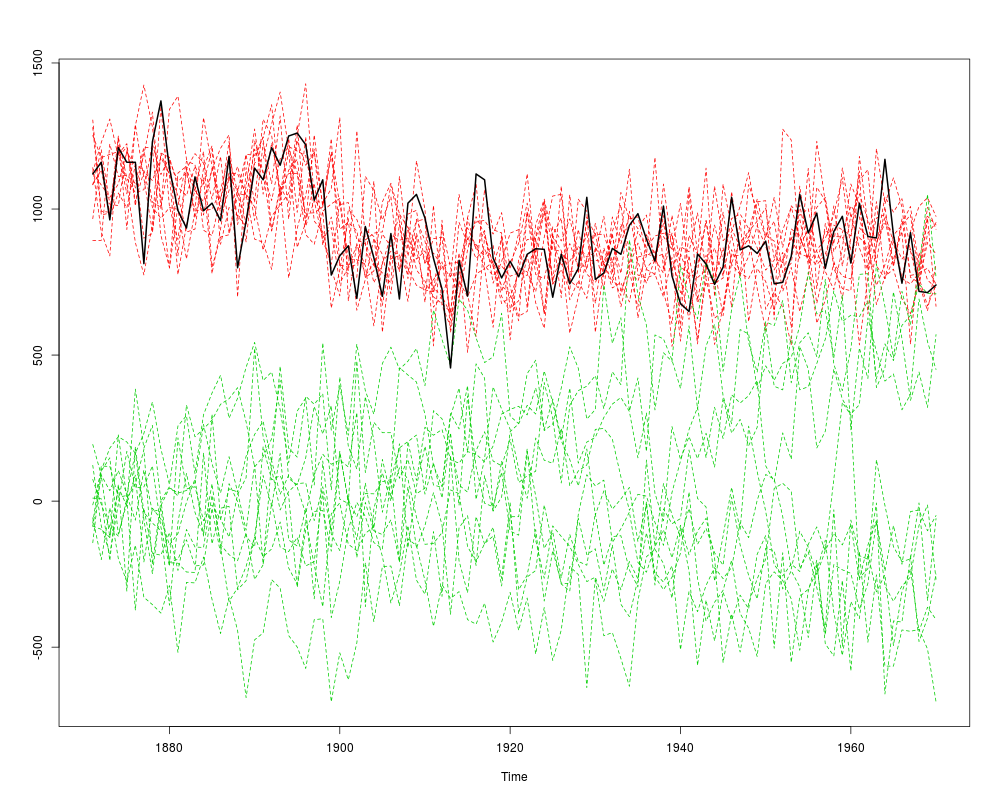
> # fully unconditional simulation:
> observation_sim2 <- simulateSSM(model, type = "observations", nsim = 10,
+ conditional = FALSE)
> ts.plot(observation_sim[,1,], observation_sim2[,1,], Nile,
+ col = c(rep(2:3, each = 10), 1), lty = c(rep(2, 20), 1),
+ lwd = c(rep(1, 20), 2))
>
> # illustrating use of antithetics
> model <- SSModel(matrix(NA, 100, 1) ~ SSMtrend(1, 1, P1inf = 0), H = 1)
>
> set.seed(123)
> sim <- simulateSSM(model, "obs", nsim = 2, antithetics = TRUE)
> # first time points
> sim[1,,]
[1] -0.07355602 -1.16865142 0.07355602 1.16865142 -0.08303054 -1.17588288
[7] 0.08303054 1.17588288
> # correlation structure between simulations with two antithetics
> cor(sim[,1,])
[,1] [,2] [,3] [,4] [,5] [,6]
[1,] 1.00000000 -0.09476707 -1.00000000 0.09476707 1.00000000 -0.09476707
[2,] -0.09476707 1.00000000 0.09476707 -1.00000000 -0.09476707 1.00000000
[3,] -1.00000000 0.09476707 1.00000000 -0.09476707 -1.00000000 0.09476707
[4,] 0.09476707 -1.00000000 -0.09476707 1.00000000 0.09476707 -1.00000000
[5,] 1.00000000 -0.09476707 -1.00000000 0.09476707 1.00000000 -0.09476707
[6,] -0.09476707 1.00000000 0.09476707 -1.00000000 -0.09476707 1.00000000
[7,] -1.00000000 0.09476707 1.00000000 -0.09476707 -1.00000000 0.09476707
[8,] 0.09476707 -1.00000000 -0.09476707 1.00000000 0.09476707 -1.00000000
[,7] [,8]
[1,] -1.00000000 0.09476707
[2,] 0.09476707 -1.00000000
[3,] 1.00000000 -0.09476707
[4,] -0.09476707 1.00000000
[5,] -1.00000000 0.09476707
[6,] 0.09476707 -1.00000000
[7,] 1.00000000 -0.09476707
[8,] -0.09476707 1.00000000
>
> out_NA <- KFS(model, filtering = "none", smoothing = "state")
> model["y"] <- sim[, 1, 1]
> out_obs <- KFS(model, filtering = "none", smoothing = "state")
>
> set.seed(40216)
> # simulate states from the p(alpha | y)
> sim_conditional <- simulateSSM(model, nsim = 10, antithetics = TRUE)
>
> # mean of the simulated states is exactly correct due to antithetic variables
> mean(sim_conditional[2, 1, ])
[1] 0.03579125
> out_obs$alpha[2]
[1] 0.03579125
> # for variances more simulations are needed
> var(sim_conditional[2, 1, ])
[1] 0.4094397
> out_obs$V[2]
[1] 0.381966
>
> set.seed(40216)
> # no data, simulations from p(alpha)
> sim_unconditional <- simulateSSM(model, nsim = 10, antithetics = TRUE,
+ conditional = FALSE)
> mean(sim_unconditional[2, 1, ])
[1] 0
> out_NA$alpha[2]
[1] 0
> var(sim_unconditional[2, 1, ])
[1] 1.300408
> out_NA$V[2]
[1] 1
>
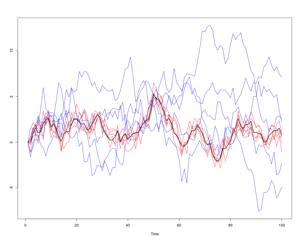
> ts.plot(cbind(sim_conditional[,1,1:5], sim_unconditional[,1,1:5]),
+ col = rep(c(2,4), each = 5))
> lines(out_obs$alpha, lwd=2)
>
>
>
>
>
>
> dev.off()
null device
1
>
|