Supported by Dr. Osamu Ogasawara and  . . |
|
Last data update: 2014.03.03 |
Kalman Filter for State Space ModelsDescriptionThese functions run the iterative equations of the Kalman filter for a state space model. UsageKF(y, ss, convergence = c(0.001, length(y)), t0 = 1) KF.C(y, ss, convergence = c(0.001, length(y)), t0 = 1) KF.deriv(y, ss, xreg = NULL, convergence = c(0.001, length(y)), t0 = 1) KF.deriv.C(y, ss, xreg = NULL, convergence = c(0.001, length(y)), t0 = 1, return.all = FALSE) Arguments
DetailsThe implementation is a direct transcription of the iterative equations of the filter that are summarized below. Details can be found in the references given below and in many other textbooks. The source code follows the notation used in Durbin and Koopman (2001). The elements in the argument The contributions to the likelihood function of the first observations
may be omitted by choosing a value of The functions with ‘ The functions Using Missing observations are allowed. If a missing value is observed after the filter has converged then all operations of the filter are run instead of using steady state values until convergence is detected again. Parameters to control the convergence of the filter.
In some models, the Kalman filter may converge to a steady state. Finding the
explicit expression of the steady state values can be cumbersome in some models.
Alternatively, at each iteration of the filter it can be checked whether a steady state
has been reached. For it, some control parameters can be defined in the argument External regressors.
A matrix of external regressors can be passed in argument The number of rows of the matrix of regressors must be equal to the length
of the series Column names are necessary for ValueA list containing the following elements:
The function The functions that evaluate the derivatives include in the output the derivatem
terms:
Derivatives of the likelihood function are implemented in package stsm. Although the Kalman filter provides information to evaluate the likelihood function, it is not its primary objective. That's why the derivatives of the likelihood are currently part of the package stsm, which is specific to likelihood methods in structural time series models. State space representationThe general univariate linear Gaussian state space model is defined as follows: y[t] = Za[t] + e[t], e[t] sim N(0, H) a[t+1] = Ta[t] + Rw[t], w[t] sim N(0, V) for t=1,…,n and a[1] sim N(a0, P0). Z is a matrix of dimension 1xm; H is 1x1; T is mxm; R is mxr; V is rxr; a0 is mx1 and P0 is mxm, where m is the dimension of the state vector a and r is the number of variance parameters in the state vector. The Kalman filtering recursions for the model above are: Prediction a[t] = T a[t-1] P[t] = T P[t-1] T' + R V R' v[t] = y[t] - Z a[t] F[t] = Z P[t] Z' + H Updating K[t] = P[t] Z' F[t]^{-1} a[t] = a[t] + K[t] v[t] P[t] = P[t] - K[t] Z P[t]' for t=2,…,n, starting with a[1] and P[1] equal
to ReferencesDurbin, J. and Koopman, S. J. (2001). Time Series Analysis by State Space Methods. Oxford University Press. Harvey, A. C. (1989). Forecasting, Structural Time Series Models and the Kalman Filter. Cambridge University Press. See Also
Examples
# local level plus seasonal model with arbitrary parameter values
# for the 'JohnsonJohnson' time series
m <- stsm::stsm.model(model = "llm+seas", y = JohnsonJohnson,
pars = c("var1" = 2, "var2" = 15, "var3" = 30))
ss <- stsm::char2numeric(m)
# run the Kalman filter
kf <- KF(m@y, ss)
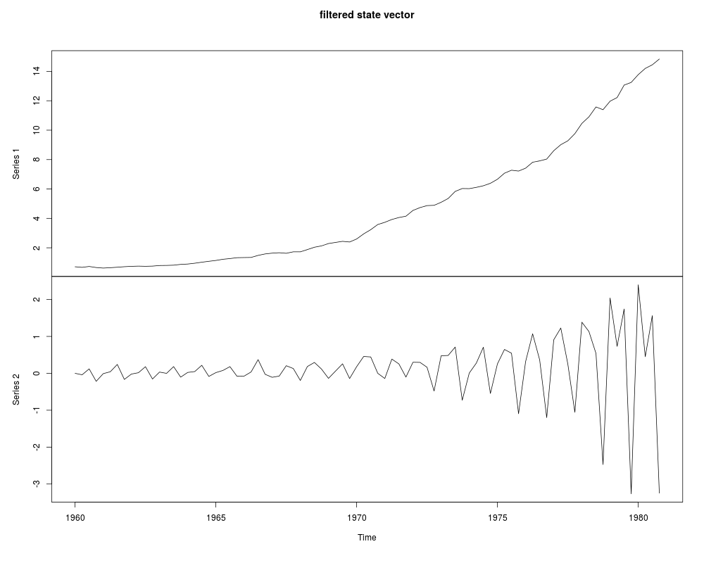
plot(kf$a.upd[,1:2], main = "filtered state vector")
# 'KF.C' is a faster version that returns only the
# value of the negative of the likelihood function
kfc <- KF.C(m@y, ss)
all.equal(kf$mll, kfc)
# compute also derivative terms used below
kfd <- KF.deriv(m@y, ss)
all.equal(kfc, kfd$mll)
kfdc <- KF.deriv.C(m@y, ss, return.all = TRUE)
all.equal(kf$mll, kfdc$mll)
# as expected the versions that use compiled C code
# are faster that the versions written fully in R
# e.g. not including derivatives
## Not run:
system.time(for(i in seq_len(10)) kf <- KF(m@y, ss))
system.time(for(i in seq_len(10)) kfc <- KF.C(m@y, ss))
# e.g. including derivatives
system.time(for(i in seq_len(10)) kfd <- KF.deriv(m@y, ss))
system.time(for(i in seq_len(10)) kfdc <- KF.deriv.C(m@y, ss, return.all = TRUE))
## End(Not run)
# compare analytical and numerical derivatives
# they give same results up to a tolerance error
fcn <- function(x, model, type = c("v", "f"))
{
m <- stsm::set.pars(model, x)
ss <- stsm::char2numeric(m)
kf <- KF(m@y, ss)
switch(type, "v" = sum(kf$v), "f" = sum(kf$f))
}
dv <- numDeriv::grad(func = fcn, x = m@pars, model = m, type = "v")
all.equal(dv, colSums(kfd$dv), check.attributes = FALSE)
all.equal(dv, colSums(kfdc$dv), check.attributes = FALSE)
df <- numDeriv::grad(func = fcn, x = m@pars, model = m, type = "f")
all.equal(df, colSums(kfd$df), check.attributes = FALSE)
all.equal(df, colSums(kfdc$df), check.attributes = FALSE)
# compare timings in version written in R with numDeriv::grad
# no calls to compiled C code in either case
# looking at these timings, using analytical derivatives is
# expected to be useful in optimization algorithms
## Not run:
system.time(for (i in seq_len(10))
numdv <- numDeriv::grad(func = fcn, x = m@pars, model = m, type = "v"))
system.time(for(i in seq_len(10)) kfdv <- colSums(KF.deriv(m@y, ss)$dv))
## End(Not run)
# compare timings when convergence is not checked with the case
# when steady state values are used after convergence is observed
# computation time is reduced substantially
## Not run:
n <- length(m@y)
system.time(for(i in seq_len(20)) a <- KF.deriv(m@y, ss, convergence = c(0.001, n)))
system.time(for(i in seq_len(20)) b <- KF.deriv(m@y, ss, convergence = c(0.001, 10)))
# the results are the same up to a tolerance error
all.equal(colSums(a$dv), colSums(b$dv))
## End(Not run)
Results
R version 3.3.1 (2016-06-21) -- "Bug in Your Hair"
Copyright (C) 2016 The R Foundation for Statistical Computing
Platform: x86_64-pc-linux-gnu (64-bit)

R is free software and comes with ABSOLUTELY NO WARRANTY.
You are welcome to redistribute it under certain conditions.
Type 'license()' or 'licence()' for distribution details.

R is a collaborative project with many contributors.
Type 'contributors()' for more information and
'citation()' on how to cite R or R packages in publications.

Type 'demo()' for some demos, 'help()' for on-line help, or
'help.start()' for an HTML browser interface to help.
Type 'q()' to quit R.

> library(KFKSDS)
> png(filename="/home/ddbj/snapshot/RGM3/R_CC/result/KFKSDS/KF.Rd_%03d_medium.png", width=480, height=480)
> ### Name: KF
> ### Title: Kalman Filter for State Space Models
> ### Aliases: KF KF.C KF.deriv KF.deriv.C
> ### Keywords: ts, model
>
> ### ** Examples
>
> # local level plus seasonal model with arbitrary parameter values
> # for the 'JohnsonJohnson' time series
> m <- stsm::stsm.model(model = "llm+seas", y = JohnsonJohnson,
+   pars = c("var1" = 2, "var2" = 15, "var3" = 30))
> ss <- stsm::char2numeric(m)
>
> # run the Kalman filter
> kf <- KF(m@y, ss)
> plot(kf$a.upd[,1:2], main = "filtered state vector")
>
> # 'KF.C' is a faster version that returns only the
> # value of the negative of the likelihood function
> kfc <- KF.C(m@y, ss)
> all.equal(kf$mll, kfc)
[1] TRUE
>
> # compute also derivative terms used below
> kfd <- KF.deriv(m@y, ss)
> all.equal(kfc, kfd$mll)
[1] TRUE
> kfdc <- KF.deriv.C(m@y, ss, return.all = TRUE)
> all.equal(kf$mll, kfdc$mll)
[1] TRUE
>
> # as expected the versions that use compiled C code
> # are faster that the versions written fully in R
> # e.g. not including derivatives
> ## Not run:
> ##D system.time(for(i in seq_len(10)) kf <- KF(m@y, ss))
> ##D system.time(for(i in seq_len(10)) kfc <- KF.C(m@y, ss))
> ##D # e.g. including derivatives
> ##D system.time(for(i in seq_len(10)) kfd <- KF.deriv(m@y, ss))
> ##D system.time(for(i in seq_len(10)) kfdc <- KF.deriv.C(m@y, ss, return.all = TRUE))
> ## End(Not run)
>
> # compare analytical and numerical derivatives
> # they give same results up to a tolerance error
> fcn <- function(x, model, type = c("v", "f"))
+ {
+   m <- stsm::set.pars(model, x)
+   ss <- stsm::char2numeric(m)
+   kf <- KF(m@y, ss)
+   switch(type, "v" = sum(kf$v), "f" = sum(kf$f))
+ }
>
> dv <- numDeriv::grad(func = fcn, x = m@pars, model = m, type = "v")
> all.equal(dv, colSums(kfd$dv), check.attributes = FALSE)
[1] TRUE
> all.equal(dv, colSums(kfdc$dv), check.attributes = FALSE)
[1] TRUE
> df <- numDeriv::grad(func = fcn, x = m@pars, model = m, type = "f")
> all.equal(df, colSums(kfd$df), check.attributes = FALSE)
[1] TRUE
> all.equal(df, colSums(kfdc$df), check.attributes = FALSE)
[1] TRUE
>
> # compare timings in version written in R with numDeriv::grad
> # no calls to compiled C code in either case
> # looking at these timings, using analytical derivatives is
> # expected to be useful in optimization algorithms
> ## Not run:
> ##D system.time(for (i in seq_len(10))
> ##D   numdv <- numDeriv::grad(func = fcn, x = m@pars, model = m, type = "v"))
> ##D system.time(for(i in seq_len(10)) kfdv <- colSums(KF.deriv(m@y, ss)$dv))
> ## End(Not run)
>
> # compare timings when convergence is not checked with the case
> # when steady state values are used after convergence is observed
> # computation time is reduced substantially
> ## Not run:
> ##D n <- length(m@y)
> ##D system.time(for(i in seq_len(20)) a <- KF.deriv(m@y, ss, convergence = c(0.001, n)))
> ##D system.time(for(i in seq_len(20)) b <- KF.deriv(m@y, ss, convergence = c(0.001, 10)))
> ##D # the results are the same up to a tolerance error
> ##D all.equal(colSums(a$dv), colSums(b$dv))
> ## End(Not run)
>
>
>
>
>
> dev.off()
null device
          1
>
|