Calculates the Distances for KNN Predictions

Description

The distances to be used for K-Nearest Neighbor (KNN) predictions are calculated and returned as a symmetric matrix. Distances are calculated by dist.

Usage

knn.dist(x, dist.meth = "euclidean", p = 2)

Arguments

Details

This function calculates the distances to be used by knn.predict. Distances are calculated between all cases. In the traditional scenario. The advantage to calculating distances in a separate step prior to prediction, is that these claculations only need to be performed once. So, for example, cross-validation to select k can be performed on many values of k, with different cross-validation splits, all using a single run of knn.dist. The default method for calculating distances is the "euclidean" distance, which is the method used by the knn function from the class package. Alternative methods may be used here. Any method valid for the function dist is valid here. The parameter p may be specified with the Minkowski distance to use the p norm as the distance method.

Value

a square symmetric matrix whose dimensions are the number of rows in the original data. The diagonal contains zeros, the off diagonal entries will be >=0..

Author(s)

Atina Dunlap Brooks

See Also

knn.predict,dist

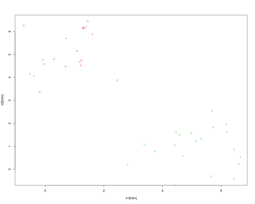
Examples

	#a quick classification example
	x1 <- c(rnorm(20, mean=1), rnorm(20, mean=5))
	x2 <- c(rnorm(20, mean=5), rnorm(20, mean=1))
	y=rep(1:2,each=20)
	x <- cbind(x1,x2)
	train <- sample(1:40, 30)
	#plot the training cases
	plot(x1[train], x2[train], col=y[train]+1)
	#predict the other cases
	test <- (1:40)[-train]
	kdist <- knn.dist(x)
	preds <- knn.predict(train, test, y ,kdist, k=3, agg.meth="majority")
	#add the predictions to the plot
	points(x1[test], x2[test], col=as.integer(preds)+1, pch="+")
	#display the confusion matrix
	table(y[test], preds)

Results

R version 3.3.1 (2016-06-21) -- "Bug in Your Hair"
Copyright (C) 2016 The R Foundation for Statistical Computing
Platform: x86_64-pc-linux-gnu (64-bit)

R is free software and comes with ABSOLUTELY NO WARRANTY.
You are welcome to redistribute it under certain conditions.
Type 'license()' or 'licence()' for distribution details.

R is a collaborative project with many contributors.
Type 'contributors()' for more information and
'citation()' on how to cite R or R packages in publications.

Type 'demo()' for some demos, 'help()' for on-line help, or
'help.start()' for an HTML browser interface to help.
Type 'q()' to quit R.

> library(KODAMA)
Loading required package: e1071
Loading required package: plsgenomics
Loading required package: MASS
Loading required package: boot
Loading required package: parallel
Loading required package: class

Attaching package: 'KODAMA'

The following object is masked from 'package:plsgenomics':

    transformy

> png(filename="/home/ddbj/snapshot/RGM3/R_CC/result/KODAMA/knn.dist.Rd_%03d_medium.png", width=480, height=480)
> ### Name: knn.dist
> ### Title: Calculates the Distances for KNN Predictions
> ### Aliases: knn.dist
> ### Keywords: distance
> 
> ### ** Examples
> 
> 	#a quick classification example
> 	x1 <- c(rnorm(20, mean=1), rnorm(20, mean=5))
> 	x2 <- c(rnorm(20, mean=5), rnorm(20, mean=1))
> 	y=rep(1:2,each=20)
> 	x <- cbind(x1,x2)
> 	train <- sample(1:40, 30)
> 	#plot the training cases
> 	plot(x1[train], x2[train], col=y[train]+1)
> 	#predict the other cases
> 	test <- (1:40)[-train]
> 	kdist <- knn.dist(x)
> 	preds <- knn.predict(train, test, y ,kdist, k=3, agg.meth="majority")
> 	#add the predictions to the plot
> 	points(x1[test], x2[test], col=as.integer(preds)+1, pch="+")
> 	#display the confusion matrix
> 	table(y[test], preds)
   preds
    1 2
  1 5 0
  2 0 5
> 
> 
> 
> 
> 
> dev.off()
null device 
          1 
>