Kernel-based Regularized Least Squares (KRLS)

Description

Function implements Kernel-Based Regularized Least Squares (KRLS), a machine learning method described in Hainmueller and Hazlett (2014) that allows users to solve regression and classification problems without manual specification search and strong functional form assumptions. KRLS finds the best fitting function by minimizing a Tikhonov regularization problem with a squared loss, using Gaussian Kernels as radial basis functions. KRLS reduces misspecification bias since it learns the functional form from the data. Yet, it nevertheless allows for interpretability and inference in ways similar to ordinary regression models. In particular, KRLS provides closed-form estimates for the predicted values, variances, and the pointwise partial derivatives that characterize the marginal effects of each independent variable at each data point in the covariate space. The distribution of pointwise marginal effects can be used to examine effect heterogeneity and or interactions.

Usage

krls(X = NULL, y = NULL, whichkernel = "gaussian", lambda = NULL,
sigma = NULL, derivative = TRUE, binary= TRUE, vcov=TRUE, 
print.level = 1,L=NULL,U=NULL,tol=NULL,eigtrunc=NULL)

Arguments

Details

krls implements the Kernel-based Regularized Least Squares (KRLS) estimator as described in Hainmueller and Hazlett (2014). Please consult this reference for any details.

Kernel-based Regularized Least Squares (KRLS) arises as a Tikhonov minimization problem with a squared loss. Assume we have data of the from y_i, x_i where i indexes observations, y_i in R is the outcome and x_i in R^D is a D-dimensional vector of predictor values. Then KRLS searches over a space of functions H and chooses the best fitting function f according to the rule:

argmin_{f in H} sum_i^N (y_i - f(x_i))^2 + lambda || f ||_H^2

where (y_i - f(x_i))^2 is a loss function that computes how ‘wrong’ the function is at each observation i and || f ||_H^2 is the regularizer that measures the complexity of the function according to the L_2 norm ||f||^2 = int f(x)^2 dx. lambda is the scalar regularization parameter that governs the tradeoff between model fit and complexity. By default, lambda is chosen by minimizing the sum of the squared leave-one-out errors, but it can also be specified by the user in the lambda argument to implement other approaches.

Under fairly general conditions, the function that minimizes the regularized loss within the hypothesis space established by the choice of a (positive semidefinite) kernel function k(x_i,x_j) is of the form

f(x_j)= sum_i^N c_i k(x_i,x_j)

where the kernel function k(x_i,x_j) measures the distance between two observations x_i and x_j and c_i is the choice coefficient for each observation i. Let K be the N by N kernel matrix with all pairwise distances K_ij=k(x_i,x_j) and c be the N by 1 vector of choice coefficients for all observations then in matrix notation the space is y=Kc.

Accordingly, the krls function solves the following minimization problem

argmin_{f in H} sum_i^n (y - Kc)'(y-Kc)+ lambda c'Kc

which is convex in c and solved by c=(K +lambda I)^-1 y where I is the identity matrix. Note that this linear solution provides a flexible fitted response surface that typically reduces misspecification bias because it can learn a wide range of nonlinear and or nonadditive functions of the predictors.

If vcov=TRUE is specified, krls also computes the variance-covariance matrix for the choice coefficients c and fitted values y=Kc based on a variance estimator developed in Hainmueller and Hazlett (2014). Note that both matrices are N by N and therefore this results in increased memory and computing time.

By default, krls uses the Gaussian Kernel (whichkernel = "gaussian") given by

k(x_i,x_j)=exp(-|| x_i - x_j ||^2 / sigma^2)

where ||x_i - x_j|| is the Euclidean distance. The kernel bandwidth sigma^2 is set to D, the number of dimensions, by default, but the user can also specify other values using the sigma argument to implement other approaches.

If derivative=TRUE is specified, krls also computes the pointwise partial derivatives of the fitted function wrt to each predictor using the estimators developed in Hainmueller and Hazlett (2014). These can be used to examine the marginal effects of each predictor and how the marginal effects vary across the covariate space. Average derivatives are also computed with variances. Note that the derivative=TRUE option results in increased computing time and is only supported for the Gaussian kernel, i.e. when whichkernel = "gaussian". Also derivative=TRUE requires that vcov=TRUE.

If binary=TRUE is also specified, the function will identify binary predictors and return first differences for these predictors instead of partial derivatives. First differences are computed going from the minimum to the maximum value of each binary predictor. Note that first differences are more appropriate to summarize the effects for binary predictors (see Hainmueller and Hazlett (2014) for details).

A few other kernels are also implemented, but derivatives are currently not supported for these: "linear": k(x_i,x_j)=x_i'x_j, "poly1", "poly2", "poly3", "poly4" are polynomial kernels based on k(x_i,x_j)=(x_i'x_j +1)^p where p is the order.

Value

A list object of class krls with the following elements:

Note

The function requires the storage of a N by N kernel matrix and can therefore exceed the memory limits for very large datasets.

Setting derivative=FALSE and vcov=FALSE is useful to reduce computing time if pointwise partial derivatives and or variance covariance matrices are not needed.

Author(s)

Jens Hainmueller (Stanford) and Chad Hazlett (MIT)

References

Hainmueller, J. and Hazlett, C. 2014.Kernel Regularized Least Squares: Reducing Misspecification Bias with a Flexible and Interpretable Machine Learning Approach. Political Analysis. (Forthcoming).

Rifkin, R. 2002. Everything Old is New Again: A fresh look at historical approaches in machine learning. Thesis, MIT. September, 2002.

Evgeniou, T., Pontil, M., and Poggio, T. (2000). Regularization networks and support vector machines. Advances In Computational Mathematics, 13(1):1-50.

Schoelkopf, B., Herbrich, R. and Smola, A.J. (2001) A generalized representer theorem. In 14th Annual Conference on Computational Learning Theory, pages 416-426.

Kimeldorf, G.S. Wahba, G. 1971. Some results on Tchebycheffian spline functions. Journal of Mathematical Analysis and Applications, 33:82-95.

See Also

predict.krls for fitted values and predictions. summary.krls for summary of the fit. plot.krls for plots of the fit.

Examples

# Linear example
# set up data
N <- 200
x1 <- rnorm(N)
x2 <- rbinom(N,size=1,prob=.2)
y <- x1 + .5*x2 + rnorm(N,0,.15)
X <- cbind(x1,x2)
# fit model
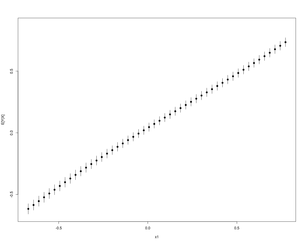
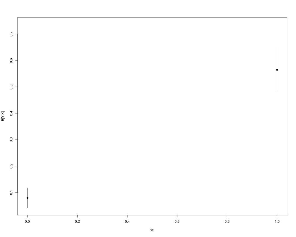
krlsout <- krls(X=X,y=y)
# summarize marginal effects and contribution of each variable
summary(krlsout)
# plot marginal effects and conditional expectation plots
plot(krlsout)


# non-linear example
# set up data
N <- 200
x1 <- rnorm(N)
x2 <- rbinom(N,size=1,prob=.2)
y <- x1^3 + .5*x2 + rnorm(N,0,.15)
X <- cbind(x1,x2)

# fit model
krlsout <- krls(X=X,y=y)
# summarize marginal effects and contribution of each variable
summary(krlsout)
# plot marginal effects and conditional expectation plots
plot(krlsout)

## 2D example:
# predictor data
X <- matrix(seq(-3,3,.1))
# true function
Ytrue <- sin(X)
# add noise 
Y     <- sin(X) + rnorm(length(X),sd=.3)
# approximate function using KRLS
out <- krls(y=Y,X=X)
# get fitted values and ses
fit <- predict(out,newdata=X,se.fit=TRUE)
# results
par(mfrow=c(2,1))
plot(y=Ytrue,x=X,type="l",col="red",ylim=c(-1.2,1.2),lwd=2,main="f(x)")
points(y=fit$fit,X,col="blue",pch=19)
arrows(y1=fit$fit+1.96*fit$se.fit,
       y0=fit$fit-1.96*fit$se.fit,
       x1=X,x0=X,col="blue",length=0)
legend("bottomright",legend=c("true f(x)=sin(x)","KRLS fitted f(x)"),
       lty=c(1,NA),pch=c(NA,19),lwd=c(2,NA),col=c("red","blue"),cex=.8)

plot(y=cos(X),x=X,type="l",col="red",ylim=c(-1.2,1.2),lwd=2,main="df(x)/dx")
points(y=out$derivatives,X,col="blue",pch=19)

legend("bottomright",legend=c("true df(x)/dx=cos(x)","KRLS fitted df(x)/dx"),
       lty=c(1,NA),pch=c(NA,19),lwd=c(2,NA),col=c("red","blue"),,cex=.8)

## 3D example
# plot true function
par(mfrow=c(1,2))
f<-function(x1,x2){ sin(x1)*cos(x2)}
x1 <- x2 <-seq(0,2*pi,.2)
z   <-outer(x1,x2,f)
persp(x1, x2, z,theta=30,main="true f(x1,x2)=sin(x1)cos(x2)")
# approximate function with KRLS
# data and outcomes
X <- cbind(sample(x1,200,replace=TRUE),sample(x2,200,replace=TRUE))
y   <- f(X[,1],X[,2])+ runif(nrow(X))
# fit surface
krlsout <- krls(X=X,y=y)
# plot fitted surface
ff  <- function(x1i,x2i,krlsout){predict(object=krlsout,newdata=cbind(x1i,x2i))$fit}
z   <- outer(x1,x2,ff,krlsout=krlsout)
persp(x1, x2, z,theta=30,main="KRLS fitted f(x1,x2)")

Results

R version 3.3.1 (2016-06-21) -- "Bug in Your Hair"
Copyright (C) 2016 The R Foundation for Statistical Computing
Platform: x86_64-pc-linux-gnu (64-bit)

R is free software and comes with ABSOLUTELY NO WARRANTY.
You are welcome to redistribute it under certain conditions.
Type 'license()' or 'licence()' for distribution details.

R is a collaborative project with many contributors.
Type 'contributors()' for more information and
'citation()' on how to cite R or R packages in publications.

Type 'demo()' for some demos, 'help()' for on-line help, or
'help.start()' for an HTML browser interface to help.
Type 'q()' to quit R.

> library(KRLS)
## KRLS Package for Kernel-based Regularized Least Squares.

## See Hainmueller and Hazlett (2014) for details.

> png(filename="/home/ddbj/snapshot/RGM3/R_CC/result/KRLS/krls.Rd_%03d_medium.png", width=480, height=480)
> ### Name: krls
> ### Title: Kernel-based Regularized Least Squares (KRLS)
> ### Aliases: krls
> ### Keywords: multivariate, smooth, kernels, machine learning, regression,
> ###   classification
> 
> ### ** Examples
> 
> 
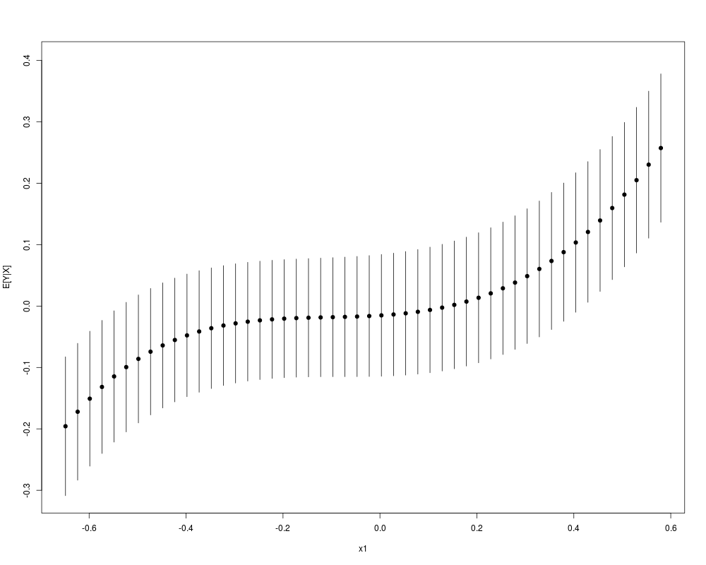
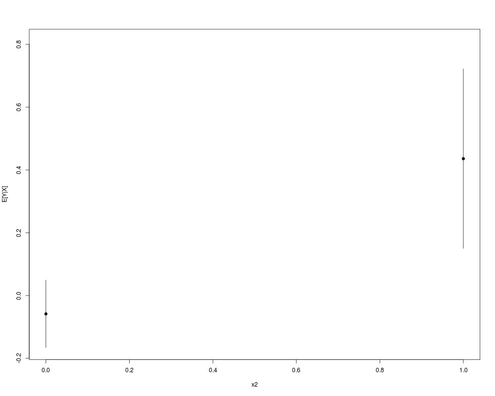
> # Linear example
> # set up data
> N <- 200
> x1 <- rnorm(N)
> x2 <- rbinom(N,size=1,prob=.2)
> y <- x1 + .5*x2 + rnorm(N,0,.15)
> X <- cbind(x1,x2)
> # fit model
> krlsout <- krls(X=X,y=y)

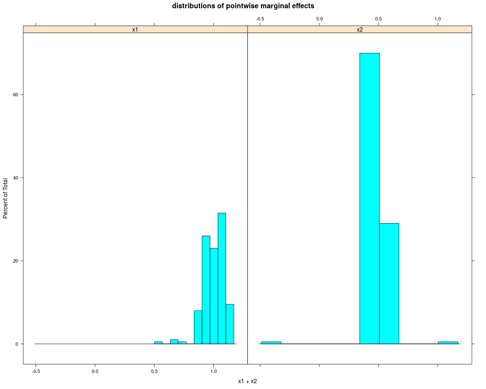
 Average Marginal Effects:
 
       x1        x2 
0.9764231 0.5177097 

 Quartiles of Marginal Effects:
 
           x1        x2
25% 0.9278731 0.4930283
50% 1.0041911 0.5149853
75% 1.0613555 0.5373586
> # summarize marginal effects and contribution of each variable
> summary(krlsout)
* *********************** *
Model Summary:

R2: 0.9761759 

Average Marginal Effects:
          Est Std. Error  t value      Pr(>|t|)
x1  0.9764231 0.01150386 84.87785 1.152751e-157
x2* 0.5177097 0.04098912 12.63042  3.295080e-27

(*) average dy/dx is for discrete change of dummy variable from min to max (i.e. usually 0 to 1))


Quartiles of Marginal Effects:
          25%       50%       75%
x1  0.9278731 1.0041911 1.0613555
x2* 0.4930283 0.5149853 0.5373586

(*) quantiles of dy/dx is for discrete change of dummy variable from min to max (i.e. usually 0 to 1))

> # plot marginal effects and conditional expectation plots
> plot(krlsout)
Loading required package: lattice
> 
> 
> # non-linear example
> # set up data
> N <- 200
> x1 <- rnorm(N)
> x2 <- rbinom(N,size=1,prob=.2)
> y <- x1^3 + .5*x2 + rnorm(N,0,.15)
> X <- cbind(x1,x2)
> 
> # fit model
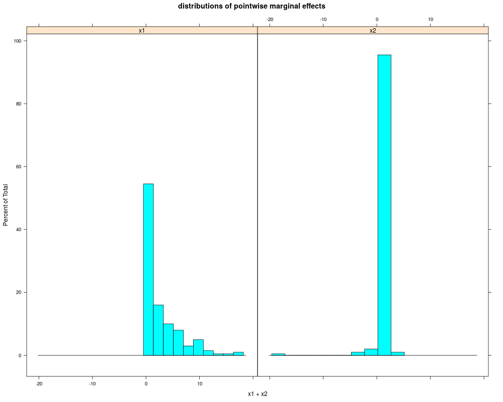
> krlsout <- krls(X=X,y=y)

 Average Marginal Effects:
 
       x1        x2 
2.7827811 0.5224141 

 Quartiles of Marginal Effects:
 
           x1        x2
25% 0.3098806 0.4954745
50% 1.1932100 0.5342347
75% 3.5015987 0.5735741
> # summarize marginal effects and contribution of each variable
> summary(krlsout)
* *********************** *
Model Summary:

R2: 0.9985203 

Average Marginal Effects:
          Est Std. Error    t value      Pr(>|t|)
x1  2.7827811 0.02555361 108.899742 1.211259e-178
x2* 0.5224141 0.08641227   6.045601  7.283638e-09

(*) average dy/dx is for discrete change of dummy variable from min to max (i.e. usually 0 to 1))


Quartiles of Marginal Effects:
          25%       50%       75%
x1  0.3098806 1.1932100 3.5015987
x2* 0.4954745 0.5342347 0.5735741

(*) quantiles of dy/dx is for discrete change of dummy variable from min to max (i.e. usually 0 to 1))

> # plot marginal effects and conditional expectation plots
> plot(krlsout)
> 
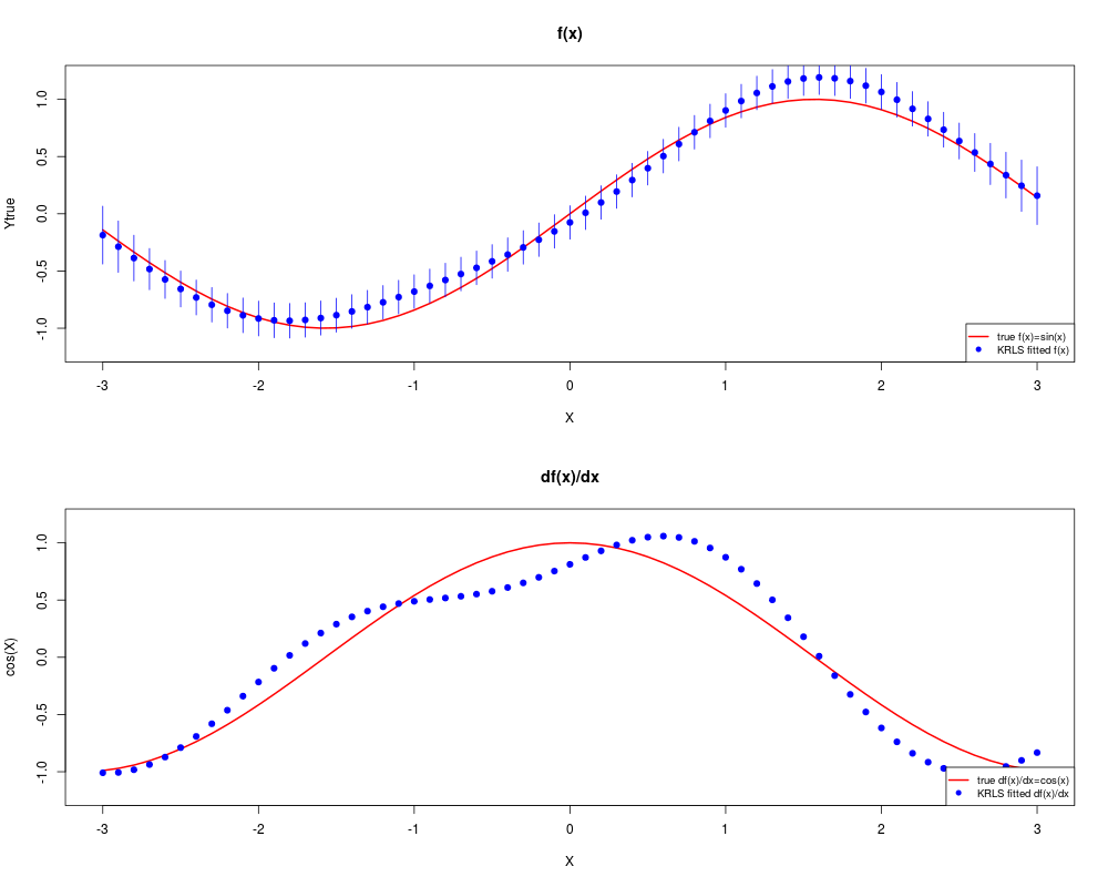
> ## 2D example:
> # predictor data
> X <- matrix(seq(-3,3,.1))
> # true function
> Ytrue <- sin(X)
> # add noise 
> Y     <- sin(X) + rnorm(length(X),sd=.3)
> # approximate function using KRLS
> out <- krls(y=Y,X=X)

 Average Marginal Effects:
 
        x1 
0.05215344 

 Quartiles of Marginal Effects:
 
            x1
25% -0.5871201
50%  0.1713179
75%  0.6582692
> # get fitted values and ses
> fit <- predict(out,newdata=X,se.fit=TRUE)
> # results
> par(mfrow=c(2,1))
> plot(y=Ytrue,x=X,type="l",col="red",ylim=c(-1.2,1.2),lwd=2,main="f(x)")
> points(y=fit$fit,X,col="blue",pch=19)
> arrows(y1=fit$fit+1.96*fit$se.fit,
+        y0=fit$fit-1.96*fit$se.fit,
+        x1=X,x0=X,col="blue",length=0)
> legend("bottomright",legend=c("true f(x)=sin(x)","KRLS fitted f(x)"),
+        lty=c(1,NA),pch=c(NA,19),lwd=c(2,NA),col=c("red","blue"),cex=.8)
> 
> plot(y=cos(X),x=X,type="l",col="red",ylim=c(-1.2,1.2),lwd=2,main="df(x)/dx")
> points(y=out$derivatives,X,col="blue",pch=19)
> 
> legend("bottomright",legend=c("true df(x)/dx=cos(x)","KRLS fitted df(x)/dx"),
+        lty=c(1,NA),pch=c(NA,19),lwd=c(2,NA),col=c("red","blue"),,cex=.8)
> 
> ## 3D example
> # plot true function
> par(mfrow=c(1,2))
> f<-function(x1,x2){ sin(x1)*cos(x2)}
> x1 <- x2 <-seq(0,2*pi,.2)
> z   <-outer(x1,x2,f)
> persp(x1, x2, z,theta=30,main="true f(x1,x2)=sin(x1)cos(x2)")
> # approximate function with KRLS
> # data and outcomes
> X <- cbind(sample(x1,200,replace=TRUE),sample(x2,200,replace=TRUE))
> y   <- f(X[,1],X[,2])+ runif(nrow(X))
> # fit surface
> krlsout <- krls(X=X,y=y)

 Average Marginal Effects:
 
         x1          x2 
-0.01670363 -0.05480133 

 Quartiles of Marginal Effects:
 
             x1          x2
25% -0.29690111 -0.41292502
50%  0.01849838 -0.04103556
75%  0.31700308  0.28816044
> # plot fitted surface
> ff  <- function(x1i,x2i,krlsout){predict(object=krlsout,newdata=cbind(x1i,x2i))$fit}
> z   <- outer(x1,x2,ff,krlsout=krlsout)
> persp(x1, x2, z,theta=30,main="KRLS fitted f(x1,x2)")
> 
> 
> 
> 
> 
> 
> dev.off()
null device 
          1 
>