R Graphical Manual

Browse All

Last data update: 2014.03.03

R: Plot method for Kernel-based Regularized Least Squares (KRLS)...

plot.krls

R Documentation

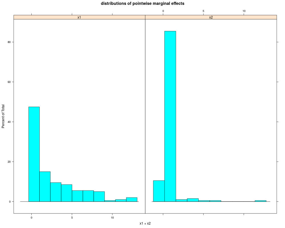
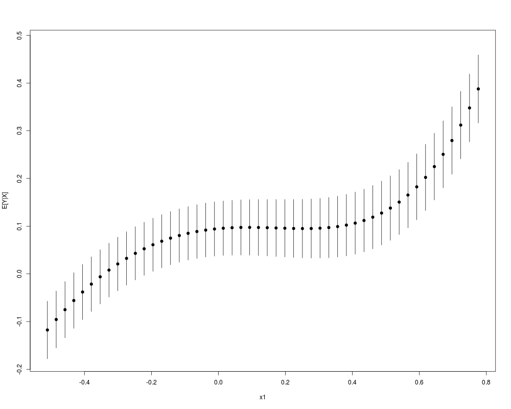
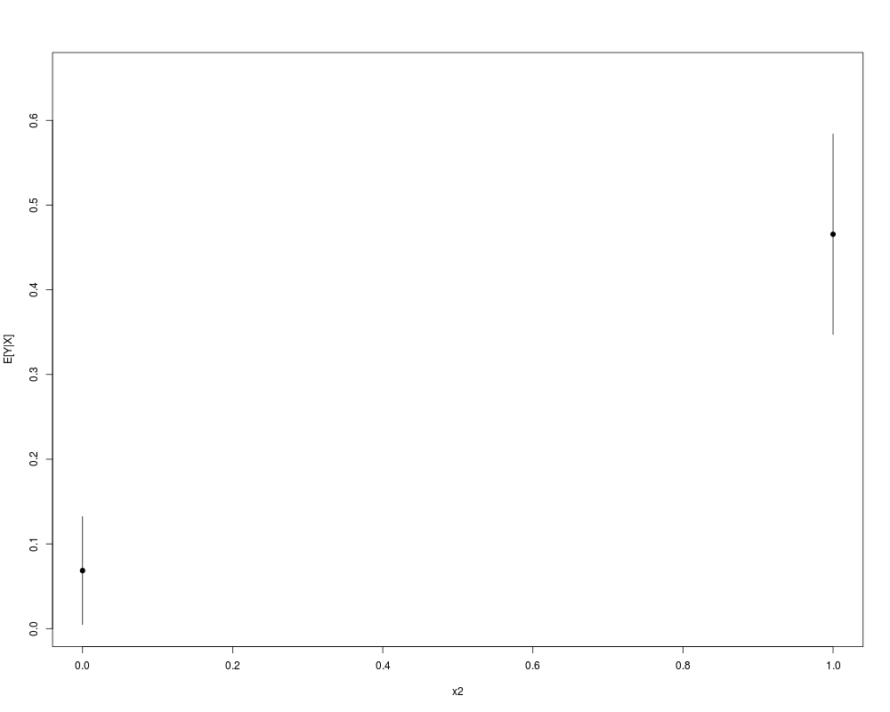
Plot method for Kernel-based Regularized Least Squares (KRLS) Model Fits

Description

Produces two types of plots. The first type of plot shows histograms for the pointwise partial derivatives to examine the heterogeneity in the marginal effects of each predictor (which==1). The second type of plot shows estimates of the conditional expectation functions of E[Y|X] for each predictor (which==2). For each plot, the predictor of interest varies from its 1st to its 3rd quartile values, while the other predictors are kept at the means (or other values specified in setx). For binary varibales the E[Y|X] are predicted at the max and the min value of the predictor (instead of the range from the 1st to the 3rd quantile).

Usage

 ## S3 method for class 'krls'
plot(x,which=c(1:2),
 main="distributions of pointwise marginal effects",
 setx="mean",ask = prod(par("mfcol")) < nplots,nvalues=50,probs=c(.25,.75),...)

Arguments

`x`	An object of class "`krls`" that results from call to `krls`.
`which`	if a subset of the plots is required, specify a subset of the numbers `1:2`.
`main`	main title for histograms of pointwise partial derivatives.
`setx`	either one of `mean` or `median` to hold other predictors at their mean or median values for the conditional expectation plots. Alternativley the user can specific a numeric vector with predictor values at which the other predictors should be fixed for the conditional expectation plots. If specifed in this way there must be one value per predictor and the order of the values much match the order of the predictor used in the predictor matrix of the krls fit passed in `x`.
`ask`	logical; if `TRUE`, the user is asked before each plot, see `par` (`ask=.`).
`nvalues`	scalar that specifies the number of values at which conditional expectations should be plotted.
`probs`	vector with numbers between 0 and 1 that specify the quantiles that determine the range for of the predictor values for which the conditional expectation should be plotted. By default we vary each predictor from the 1st quartile to the 3rd quartile value.
`...`	additional arguments to be passed to lower level functions

Details

Notice that the historgrams for the partial derivatives can only be plotted if the KRLS object was computed with krls(,derivatives=TRUE).

Author(s)

Jens Hainmueller (Stanford) and Chad Hazlett (MIT)

Examples

# non-linear example
# set up data
N <- 200
x1 <- rnorm(N)
x2 <- rbinom(N,size=1,prob=.2)
y <- x1^3 + .5*x2 + rnorm(N,0,.15)
X <- cbind(x1,x2)

# fit model
krlsout <- krls(X=X,y=y)
# summarize marginal effects and contribution of each variable
summary(krlsout)
# plot marginal effects and conditional expectation plots
plot(krlsout)

Results


R version 3.3.1 (2016-06-21) -- "Bug in Your Hair"
Copyright (C) 2016 The R Foundation for Statistical Computing
Platform: x86_64-pc-linux-gnu (64-bit)

R is free software and comes with ABSOLUTELY NO WARRANTY.
You are welcome to redistribute it under certain conditions.
Type 'license()' or 'licence()' for distribution details.

R is a collaborative project with many contributors.
Type 'contributors()' for more information and
'citation()' on how to cite R or R packages in publications.

Type 'demo()' for some demos, 'help()' for on-line help, or
'help.start()' for an HTML browser interface to help.
Type 'q()' to quit R.

> library(KRLS)
## KRLS Package for Kernel-based Regularized Least Squares.

## See Hainmueller and Hazlett (2014) for details.

> png(filename="/home/ddbj/snapshot/RGM3/R_CC/result/KRLS/plot.krls.Rd_%03d_medium.png", width=480, height=480)
> ### Name: plot.krls
> ### Title: Plot method for Kernel-based Regularized Least Squares (KRLS)
> ###   Model Fits
> ### Aliases: plot.krls
> 
> ### ** Examples
> 
> # non-linear example
> # set up data
> N <- 200
> x1 <- rnorm(N)
> x2 <- rbinom(N,size=1,prob=.2)
> y <- x1^3 + .5*x2 + rnorm(N,0,.15)
> X <- cbind(x1,x2)
> 
> # fit model
> krlsout <- krls(X=X,y=y)

 Average Marginal Effects:
 
       x1        x2 
3.3126330 0.9462857 

 Quartiles of Marginal Effects:
 
           x1        x2
25% 0.3852749 0.4157484
50% 1.4182534 0.5190885
75% 4.5737327 0.6040110
> # summarize marginal effects and contribution of each variable
> summary(krlsout)
* *********************** *
Model Summary:

R2: 0.9946028 

Average Marginal Effects:
          Est Std. Error   t value      Pr(>|t|)
x1  3.3126330 0.02600654 127.37692 6.252267e-192
x2* 0.9462857 0.09075319  10.42702  1.433487e-20

(*) average dy/dx is for discrete change of dummy variable from min to max (i.e. usually 0 to 1))


Quartiles of Marginal Effects:
          25%       50%      75%
x1  0.3852749 1.4182534 4.573733
x2* 0.4157484 0.5190885 0.604011

(*) quantiles of dy/dx is for discrete change of dummy variable from min to max (i.e. usually 0 to 1))

> # plot marginal effects and conditional expectation plots
> plot(krlsout)
Loading required package: lattice
> 
> 
> 
> 
> 
> 
> dev.off()
null device 
          1 
>