KScorrect: Lilliefors-Corrected Kolmogorov-Smirnoff Goodness-of-Fit Tests

Description

Implements the Lilliefors-corrected Kolmogorov-Smirnoff test for use in goodness-of-fit tests.

Details

KScorrect implements the Lilliefors-corrected Kolmogorov-Smirnoff test for use in goodness-of-fit tests, suitable when population parameters are unknown and must be estimated by sample statistics. P-values are estimated by simulation. Coded to complement ks.test, it can be used with a variety of continuous distributions, including normal, lognormal, univariate mixtures of normals, uniform, loguniform, exponential, gamma, and Weibull distributions.

Functions to generate random numbers and calculate density, distribution, and quantile functions are provided for use with the loguniform and mixture distributions.

Author(s)

Phil Novack-Gottshall pnovack-gottshall@ben.edu

Steve C. Wang scwang@swarthmore.edu

Examples

# Get the package version and citation of KScorrect
packageVersion("KScorrect")
citation("KScorrect")

x <- runif(200)
Lc <- LcKS(x, cdf="pnorm", nreps=999)
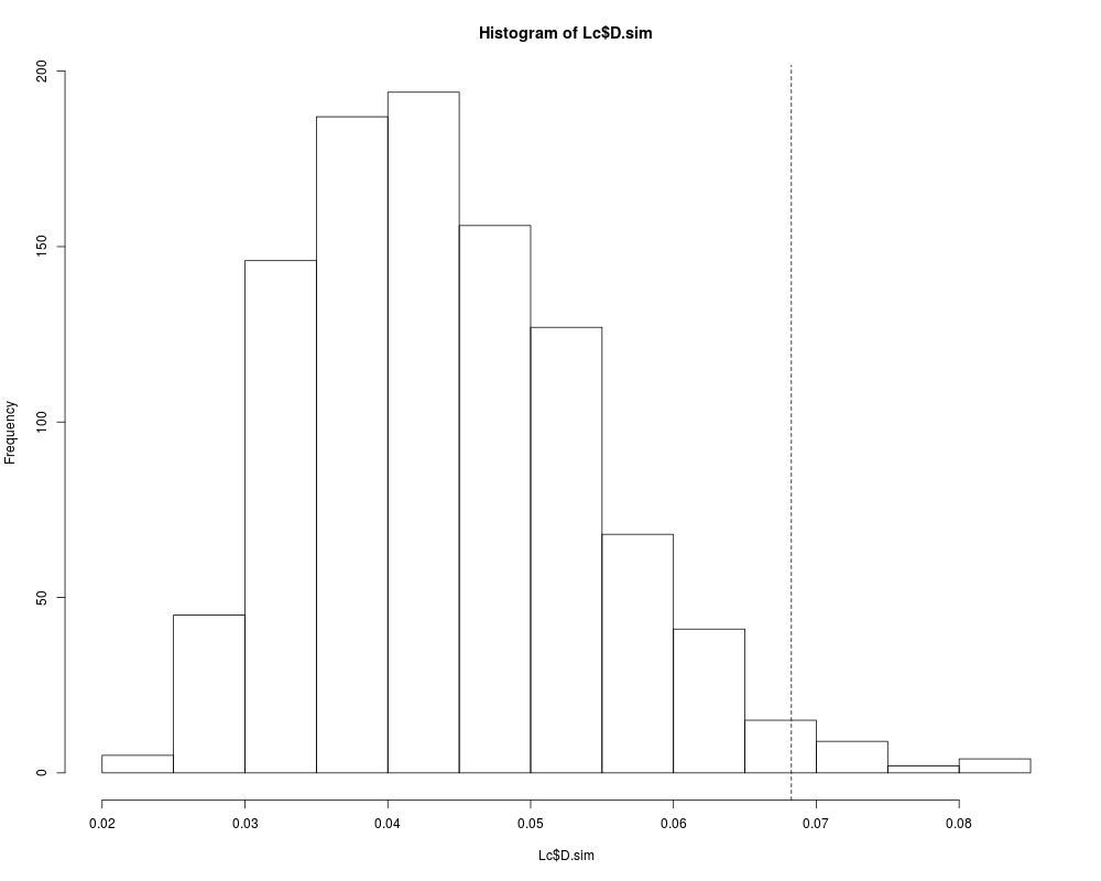
hist(Lc$D.sim)
abline(v = Lc$D.obs, lty = 2)
print(Lc, max=50)  # Print first 50 simulated statistics
# Approximate p-value (usually) << 0.05

# Confirmation uncorrected version has increased Type II error rate when
#   using sample statistics to estimate parameters:
ks.test(x, "pnorm", mean(x), sd(x))   # p-value always larger, (usually) > 0.05

x <- rlunif(200, min=exp(1), max=exp(10)) # random loguniform sample
Lc <- LcKS(x, cdf="plnorm")
Lc$p.value      # Approximate p-value: (usually) << 0.05

Results

R version 3.3.1 (2016-06-21) -- "Bug in Your Hair"
Copyright (C) 2016 The R Foundation for Statistical Computing
Platform: x86_64-pc-linux-gnu (64-bit)

R is free software and comes with ABSOLUTELY NO WARRANTY.
You are welcome to redistribute it under certain conditions.
Type 'license()' or 'licence()' for distribution details.

R is a collaborative project with many contributors.
Type 'contributors()' for more information and
'citation()' on how to cite R or R packages in publications.

Type 'demo()' for some demos, 'help()' for on-line help, or
'help.start()' for an HTML browser interface to help.
Type 'q()' to quit R.

> library(KScorrect)
> png(filename="/home/ddbj/snapshot/RGM3/R_CC/result/KScorrect/KScorrect-package.Rd_%03d_medium.png", width=480, height=480)
> ### Name: KScorrect-package
> ### Title: KScorrect: Lilliefors-Corrected Kolmogorov-Smirnoff
> ###   Goodness-of-Fit Tests
> ### Aliases: KScorrect KScorrect-package
> 
> ### ** Examples
> 
> # Get the package version and citation of KScorrect
> packageVersion("KScorrect")
[1] '1.2.0'
> citation("KScorrect")

To cite package 'KScorrect' in publications use:

  Phil Novack-Gottshall and Steve C. Wang (2016). KScorrect:
  Lilliefors-Corrected Kolmogorov-Smirnoff Goodness-of-Fit Tests. R
  package version 1.2.0. https://CRAN.R-project.org/package=KScorrect

A BibTeX entry for LaTeX users is

  @Manual{,
    title = {KScorrect: Lilliefors-Corrected Kolmogorov-Smirnoff Goodness-of-Fit Tests},
    author = {Phil Novack-Gottshall and Steve C. Wang},
    year = {2016},
    note = {R package version 1.2.0},
    url = {https://CRAN.R-project.org/package=KScorrect},
  }

ATTENTION: This citation information has been auto-generated from the
package DESCRIPTION file and may need manual editing, see
'help("citation")'.

> 
> x <- runif(200)
> Lc <- LcKS(x, cdf="pnorm", nreps=999)
> hist(Lc$D.sim)
> abline(v = Lc$D.obs, lty = 2)
> print(Lc, max=50)  # Print first 50 simulated statistics
$D.obs
[1] 0.09040818

$D.sim
 [1] 0.03133192 0.05120694 0.05499319 0.03139640 0.03865632 0.05973092
 [7] 0.04897101 0.06346032 0.03371124 0.03928754 0.04186174 0.04580865
[13] 0.06534087 0.03602895 0.03662798 0.03423945 0.03067187 0.04693140
[19] 0.03661235 0.03485921 0.05850112 0.06856553 0.04127479 0.04806951
[25] 0.03813411 0.03376392 0.04179635 0.05027615 0.03656406 0.04024797
[31] 0.04431635 0.05284283 0.03543756 0.04380115 0.03393701 0.05153280
[37] 0.04221833 0.04178663 0.05700971 0.03623534 0.04709811 0.02501283
[43] 0.05272168 0.04129674 0.04232167 0.04663018 0.03618791 0.03438787
[49] 0.04052766 0.05908228
 [ reached getOption("max.print") -- omitted 949 entries ]

$p.value
[1] 0.001

> # Approximate p-value (usually) << 0.05
> 
> # Confirmation uncorrected version has increased Type II error rate when
> #   using sample statistics to estimate parameters:
> ks.test(x, "pnorm", mean(x), sd(x))   # p-value always larger, (usually) > 0.05

	One-sample Kolmogorov-Smirnov test

data:  x
D = 0.090408, p-value = 0.07605
alternative hypothesis: two-sided

> 
> x <- rlunif(200, min=exp(1), max=exp(10)) # random loguniform sample
> Lc <- LcKS(x, cdf="plnorm")
> Lc$p.value      # Approximate p-value: (usually) << 0.05
[1] 0.0048
> 
> 
> 
> 
> 
> dev.off()
null device 
          1 
>