Supported by Dr. Osamu Ogasawara and  . . |
|
Last data update: 2014.03.03 |
Compute a 2D Binned Kernel Density EstimateDescriptionReturns the set of grid points in each coordinate direction, and the matrix of density estimates over the mesh induced by the grid points. The kernel is the standard bivariate normal density. Usagebkde2D(x, bandwidth, gridsize = c(51L, 51L), range.x, truncate = TRUE) Arguments
Valuea list containing the following components:
DetailsThis is the binned approximation to the 2D kernel density estimate.
Linear binning is used to obtain the bin counts and the
Fast Fourier Transform is used to perform the discrete convolutions.
For each ReferencesWand, M. P. (1994). Fast Computation of Multivariate Kernel Estimators. Journal of Computational and Graphical Statistics, 3, 433-445. Wand, M. P. and Jones, M. C. (1995). Kernel Smoothing. Chapman and Hall, London. See Also
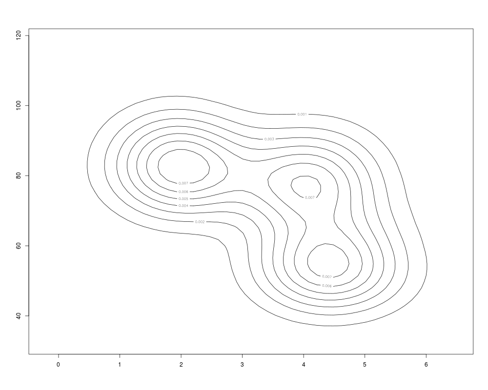
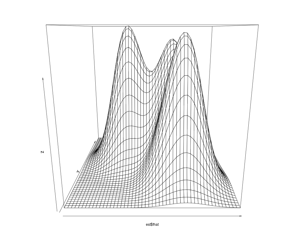
Examplesdata(geyser, package="MASS") x <- cbind(geyser$duration, geyser$waiting) est <- bkde2D(x, bandwidth=c(0.7, 7)) contour(est$x1, est$x2, est$fhat) persp(est$fhat) Results
R version 3.3.1 (2016-06-21) -- "Bug in Your Hair"
Copyright (C) 2016 The R Foundation for Statistical Computing
Platform: x86_64-pc-linux-gnu (64-bit)

R is free software and comes with ABSOLUTELY NO WARRANTY.
You are welcome to redistribute it under certain conditions.
Type 'license()' or 'licence()' for distribution details.

R is a collaborative project with many contributors.
Type 'contributors()' for more information and
'citation()' on how to cite R or R packages in publications.

Type 'demo()' for some demos, 'help()' for on-line help, or
'help.start()' for an HTML browser interface to help.
Type 'q()' to quit R.

> library(KernSmooth)
KernSmooth 2.23 loaded
Copyright M. P. Wand 1997-2009
> png(filename="/home/ddbj/snapshot/RGM3/R_CC/result/KernSmooth/bkde2D.Rd_%03d_medium.png", width=480, height=480)
> ### Name: bkde2D
> ### Title: Compute a 2D Binned Kernel Density Estimate
> ### Aliases: bkde2D
> ### Keywords: distribution smooth
>
> ### ** Examples
>
> data(geyser, package="MASS")
> x <- cbind(geyser$duration, geyser$waiting)
> est <- bkde2D(x, bandwidth=c(0.7, 7))
> contour(est$x1, est$x2, est$fhat)
> persp(est$fhat)
>
>
>
>
>
> dev.off()
null device
          1
>
|