Quick computation of kriging covariances

Description

Computes kriging covariances between one new point and many integration points, using precomputed data.

Usage

computeQuickKrigcov(model,integration.points,X.new,
precalc.data, F.newdata , c.newdata)

Arguments

Details

This function requires to use another function in order to generate the proper arguments. The argument precalc.data can be generated using precomputeUpdateData. The arguments F.newdata and c.newdata can be obtained using predict_nobias_km, which returns a field F.newdata and a field c.

Value

A vector containing kriging covariances

Author(s)

Clement Chevalier (IMSV, Switzerland, and IRSN, France)

References

Chevalier C., Bect J., Ginsbourger D., Vazquez E., Picheny V., Richet Y. (2011), Fast parallel kriging-based stepwise uncertainty reduction with application to the identification of an excursion set ,http://hal.archives-ouvertes.fr/hal-00641108/

Chevalier C., Ginsbourger D. (2012), Corrected Kriging update formulae for batch-sequential data assimilation ,http://arxiv.org/pdf/1203.6452.pdf

See Also

precomputeUpdateData, predict_nobias_km, predict_update_km

Examples

#computeQuickKrigcov

set.seed(8)
N <- 9 #number of observations
testfun <- branin

#a 9 points initial design
design <- data.frame( matrix(runif(2*N),ncol=2) )
response <- testfun(design)

#km object with matern3_2 covariance
#params estimated by ML from the observations
model <- km(formula=~., design = design, 
	response = response,covtype="matern3_2")

#the points where we want to compute prediction 
#if a point new.x is added to the doe
n.grid <- 20 #you can run it with 100
x.grid <- y.grid <- seq(0,1,length=n.grid)
newdata <- expand.grid(x.grid,y.grid)

#precalculation
precalc.data <- precomputeUpdateData(model=model,
		integration.points=newdata)

#now we can compute very quickly kriging covariances 
#between these data and any other points
other.x <- matrix(c(0.6,0.6),ncol=2)
pred <- predict_nobias_km(object=model,
	newdata=other.x,type="UK",se.compute=TRUE)

kn <- computeQuickKrigcov(model=model,
	integration.points=newdata,X.new=other.x,
        precalc.data=precalc.data,
	F.newdata=pred$F.newdata,
        c.newdata=pred$c)

z.grid <- matrix(kn, n.grid, n.grid)

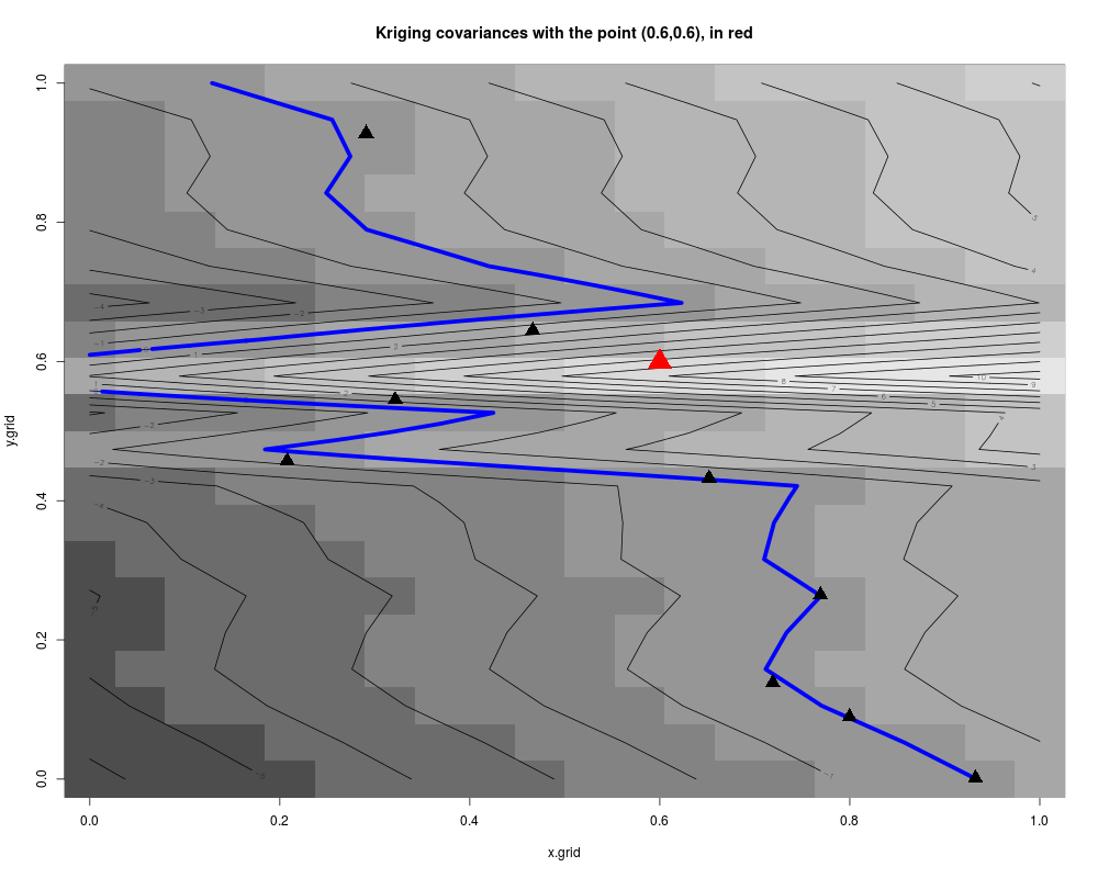
#plots: contour of the criterion, doe points and new point
image(x=x.grid,y=y.grid,z=z.grid,col=grey.colors(10))
contour(x=x.grid,y=y.grid,z=z.grid,15,add=TRUE)
contour(x=x.grid,y=y.grid,z=z.grid,levels=0,add=TRUE,col="blue",lwd=5)
points(design, col="black", pch=17, lwd=4,cex=2)
points(other.x, col="red", pch=17, lwd=4,cex=3)
title("Kriging covariances with the point (0.6,0.6), in red")

Results

R version 3.3.1 (2016-06-21) -- "Bug in Your Hair"
Copyright (C) 2016 The R Foundation for Statistical Computing
Platform: x86_64-pc-linux-gnu (64-bit)

R is free software and comes with ABSOLUTELY NO WARRANTY.
You are welcome to redistribute it under certain conditions.
Type 'license()' or 'licence()' for distribution details.

R is a collaborative project with many contributors.
Type 'contributors()' for more information and
'citation()' on how to cite R or R packages in publications.

Type 'demo()' for some demos, 'help()' for on-line help, or
'help.start()' for an HTML browser interface to help.
Type 'q()' to quit R.

> library(KrigInv)
Loading required package: DiceKriging
Loading required package: pbivnorm
Loading required package: rgenoud
##  rgenoud (Version 5.7-12.4, Build Date: 2015-07-19)
##  See http://sekhon.berkeley.edu/rgenoud for additional documentation.
##  Please cite software as:
##   Walter Mebane, Jr. and Jasjeet S. Sekhon. 2011.
##   ``Genetic Optimization Using Derivatives: The rgenoud package for R.''
##   Journal of Statistical Software, 42(11): 1-26. 
##

Loading required package: randtoolbox
Loading required package: rngWELL
This is randtoolbox. For overview, type 'help("randtoolbox")'.
> png(filename="/home/ddbj/snapshot/RGM3/R_CC/result/KrigInv/computeQuickKrigcov.Rd_%03d_medium.png", width=480, height=480)
> ### Name: computeQuickKrigcov
> ### Title: Quick computation of kriging covariances
> ### Aliases: computeQuickKrigcov
> 
> ### ** Examples
> 
> #computeQuickKrigcov
> 
> set.seed(8)
> N <- 9 #number of observations
> testfun <- branin
> 
> #a 9 points initial design
> design <- data.frame( matrix(runif(2*N),ncol=2) )
> response <- testfun(design)
> 
> #km object with matern3_2 covariance
> #params estimated by ML from the observations
> model <- km(formula=~., design = design, 
+ 	response = response,covtype="matern3_2")

optimisation start
------------------
* estimation method   : MLE 
* optimisation method : BFGS 
* analytical gradient : used
* trend model : ~X1 + X2
* covariance model : 
  - type :  matern3_2 
  - nugget : NO
  - parameters lower bounds :  1e-10 1e-10 
  - parameters upper bounds :  1.448893 1.853021 
  - best initial criterion value(s) :  -25.38168 

N = 2, M = 5 machine precision = 2.22045e-16
At X0, 0 variables are exactly at the bounds
At iterate     0  f=       25.382  |proj g|=      0.19431
At iterate     1  f =       25.027  |proj g|=       0.13259
At iterate     2  f =       25.014  |proj g|=        1.6725
At iterate     3  f =       25.002  |proj g|=       0.15969
At iterate     4  f =       25.001  |proj g|=       0.17792
At iterate     5  f =       24.999  |proj g|=       0.31318
At iterate     6  f =       24.998  |proj g|=       0.14968
At iterate     7  f =       24.998  |proj g|=       0.03446
At iterate     8  f =       24.998  |proj g|=       0.03458
At iterate     9  f =       24.998  |proj g|=     0.0084816
At iterate    10  f =       24.998  |proj g|=      0.038393
At iterate    11  f =       24.997  |proj g|=        1.3196
At iterate    12  f =       24.997  |proj g|=        1.3327
At iterate    13  f =       24.994  |proj g|=        1.8077
At iterate    14  f =       24.991  |proj g|=        1.8106
At iterate    15  f =       24.975  |proj g|=        1.8136
At iterate    16  f =       24.937  |proj g|=        1.8202
At iterate    17  f =       24.816  |proj g|=        1.8136
At iterate    18  f =       24.652  |proj g|=       0.81261
At iterate    19  f =       24.652  |proj g|=       0.25743
At iterate    20  f =       24.651  |proj g|=     0.0033442
At iterate    21  f =       24.651  |proj g|=    1.4045e-05

iterations 21
function evaluations 30
segments explored during Cauchy searches 22
BFGS updates skipped 0
active bounds at final generalized Cauchy point 1
norm of the final projected gradient 1.40447e-05
final function value 24.6515

F = 24.6515
final  value 24.651471 
converged
> 
> #the points where we want to compute prediction 
> #if a point new.x is added to the doe
> n.grid <- 20 #you can run it with 100
> x.grid <- y.grid <- seq(0,1,length=n.grid)
> newdata <- expand.grid(x.grid,y.grid)
> 
> #precalculation
> precalc.data <- precomputeUpdateData(model=model,
+ 		integration.points=newdata)
> 
> #now we can compute very quickly kriging covariances 
> #between these data and any other points
> other.x <- matrix(c(0.6,0.6),ncol=2)
> pred <- predict_nobias_km(object=model,
+ 	newdata=other.x,type="UK",se.compute=TRUE)
> 
> kn <- computeQuickKrigcov(model=model,
+ 	integration.points=newdata,X.new=other.x,
+         precalc.data=precalc.data,
+ 	F.newdata=pred$F.newdata,
+         c.newdata=pred$c)
> 
> z.grid <- matrix(kn, n.grid, n.grid)
> 
> #plots: contour of the criterion, doe points and new point
> image(x=x.grid,y=y.grid,z=z.grid,col=grey.colors(10))
> contour(x=x.grid,y=y.grid,z=z.grid,15,add=TRUE)
> contour(x=x.grid,y=y.grid,z=z.grid,levels=0,add=TRUE,col="blue",lwd=5)
> points(design, col="black", pch=17, lwd=4,cex=2)
> points(other.x, col="red", pch=17, lwd=4,cex=3)
> title("Kriging covariances with the point (0.6,0.6), in red")
> 
> 
> 
> 
> 
> dev.off()
null device 
          1 
>