Supported by Dr. Osamu Ogasawara and  . . |
|
Last data update: 2014.03.03 |
Construction of a sample of integration points and weightsDescriptionGeneric function to build integration points for some sampling criterion.
Available important sampling schemes are Usageintegration_design(integcontrol = NULL, d = NULL, lower, upper, model = NULL, T = NULL,min.prob=0.001) Arguments
DetailsThe important sampling aims at improving the accuracy of the calculation of numerical integrals present in these criteria. ValueA list with components:
Author(s)Clement Chevalier (IMSV, Switzerland, and IRSN, France) ReferencesChevalier C., Picheny V., Ginsbourger D. (2012), The KrigInv package: An efficient and user-friendly R implementation of Kriging-based inversion algorithms , http://hal.archives-ouvertes.fr/hal-00713537/ Chevalier C., Bect J., Ginsbourger D., Vazquez E., Picheny V., Richet Y. (2011), Fast parallel kriging-based stepwise uncertainty reduction with application to the identification of an excursion set ,http://hal.archives-ouvertes.fr/hal-00641108/ Bect J., Ginsbourger D., Li L., Picheny V., Vazquez E. (2010), Sequential design of computer experiments for the estimation of a probability of failure, Statistics and Computing, pp.1-21, 2011, http://arxiv.org/abs/1009.5177 See Also
Examples#integration_design ## Not run: set.seed(8) #when nothing is specified: integration points #are chosen with the sobol sequence integ.param <- integration_design(lower=c(0,0),upper=c(1,1)) plot(integ.param$integration.points) ## End(Not run) #an example with pure random integration points integcontrol <- list(distrib="MC",n.points=50) integ.param <- integration_design(integcontrol=integcontrol, lower=c(0,0),upper=c(1,1)) plot(integ.param$integration.points) #an example with important sampling distributions #these distributions are used to compute integral criterion like #"sur","timse" or "imse" #for these, we need a kriging model N <- 14;testfun <- branin; T <- 80 lower <- c(0,0);upper <- c(1,1) design <- data.frame( matrix(runif(2*N),ncol=2) ) response <- testfun(design) model <- km(formula=~., design = design, response = response,covtype="matern3_2") integcontrol <- list(distrib="timse",n.points=200,n.candidates=5000,init.distrib="MC") integ.param <- integration_design(integcontrol=integcontrol, lower=c(0,0),upper=c(1,1), model=model,T=T) print_uncertainty_2d(model=model,T=T,type="timse", col.points.init="red",cex.points=2, main="timse uncertainty and one sample of integration points") points(integ.param$integration.points,pch=17,cex=1) Results
R version 3.3.1 (2016-06-21) -- "Bug in Your Hair"
Copyright (C) 2016 The R Foundation for Statistical Computing
Platform: x86_64-pc-linux-gnu (64-bit)
R is free software and comes with ABSOLUTELY NO WARRANTY.
You are welcome to redistribute it under certain conditions.
Type 'license()' or 'licence()' for distribution details.
R is a collaborative project with many contributors.
Type 'contributors()' for more information and
'citation()' on how to cite R or R packages in publications.
Type 'demo()' for some demos, 'help()' for on-line help, or
'help.start()' for an HTML browser interface to help.
Type 'q()' to quit R.
> library(KrigInv)
Loading required package: DiceKriging
Loading required package: pbivnorm
Loading required package: rgenoud
## rgenoud (Version 5.7-12.4, Build Date: 2015-07-19)
## See http://sekhon.berkeley.edu/rgenoud for additional documentation.
## Please cite software as:
## Walter Mebane, Jr. and Jasjeet S. Sekhon. 2011.
## ``Genetic Optimization Using Derivatives: The rgenoud package for R.''
## Journal of Statistical Software, 42(11): 1-26.
##
Loading required package: randtoolbox
Loading required package: rngWELL
This is randtoolbox. For overview, type 'help("randtoolbox")'.
> png(filename="/home/ddbj/snapshot/RGM3/R_CC/result/KrigInv/integration_design.Rd_%03d_medium.png", width=480, height=480)
> ### Name: integration_design
> ### Title: Construction of a sample of integration points and weights
> ### Aliases: integration_design
>
> ### ** Examples
>
> #integration_design
>
> ## Not run:
> ##D set.seed(8)
> ##D #when nothing is specified: integration points
> ##D #are chosen with the sobol sequence
> ##D integ.param <- integration_design(lower=c(0,0),upper=c(1,1))
> ##D plot(integ.param$integration.points)
> ## End(Not run)
>
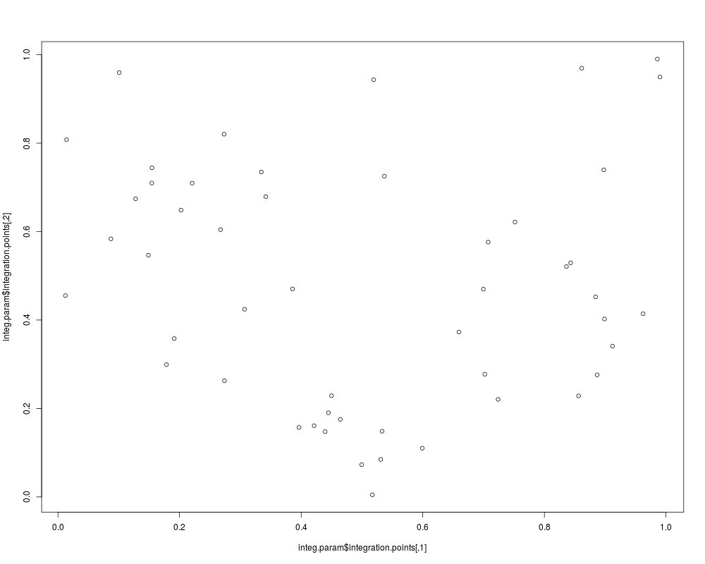
> #an example with pure random integration points
> integcontrol <- list(distrib="MC",n.points=50)
> integ.param <- integration_design(integcontrol=integcontrol,
+ lower=c(0,0),upper=c(1,1))
> plot(integ.param$integration.points)
>
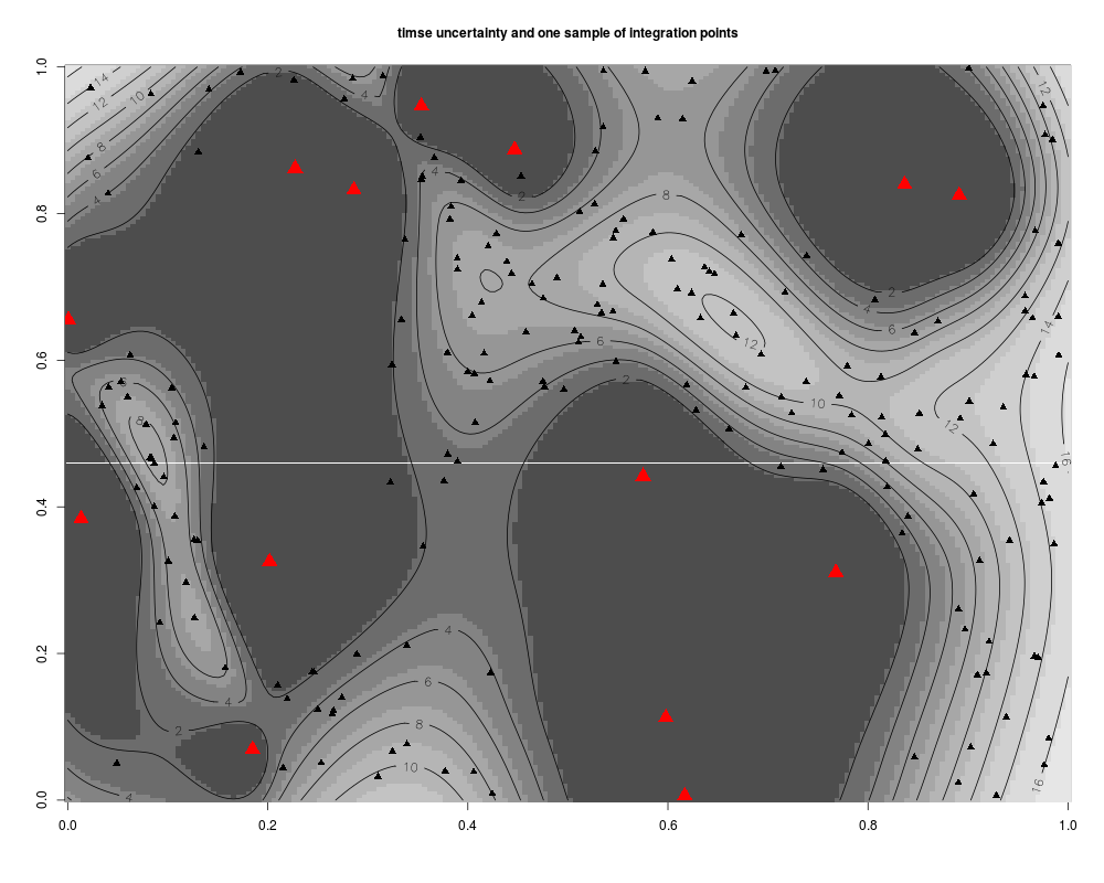
> #an example with important sampling distributions
> #these distributions are used to compute integral criterion like
> #"sur","timse" or "imse"
>
> #for these, we need a kriging model
> N <- 14;testfun <- branin; T <- 80
> lower <- c(0,0);upper <- c(1,1)
> design <- data.frame( matrix(runif(2*N),ncol=2) )
> response <- testfun(design)
> model <- km(formula=~., design = design,
+ response = response,covtype="matern3_2")
optimisation start
------------------
* estimation method : MLE
* optimisation method : BFGS
* analytical gradient : used
* trend model : ~X1 + X2
* covariance model :
- type : matern3_2
- nugget : NO
- parameters lower bounds : 1e-10 1e-10
- parameters upper bounds : 1.66491 1.36074
- best initial criterion value(s) : -58.19104
N = 2, M = 5 machine precision = 2.22045e-16
At X0, 0 variables are exactly at the bounds
At iterate 0 f= 58.191 |proj g|= 1.2118
At iterate 1 f = 57.639 |proj g|= 1.5358
At iterate 2 f = 56.537 |proj g|= 1.4467
At iterate 3 f = 56.458 |proj g|= 1.0719
At iterate 4 f = 56.452 |proj g|= 0.17712
At iterate 5 f = 56.451 |proj g|= 0.14418
At iterate 6 f = 56.45 |proj g|= 0.049361
At iterate 7 f = 56.45 |proj g|= 0.0012268
At iterate 8 f = 56.45 |proj g|= 2.8078e-06
iterations 8
function evaluations 10
segments explored during Cauchy searches 9
BFGS updates skipped 0
active bounds at final generalized Cauchy point 0
norm of the final projected gradient 2.8078e-06
final function value 56.4501
F = 56.4501
final value 56.450079
converged
>
> integcontrol <- list(distrib="timse",n.points=200,n.candidates=5000,init.distrib="MC")
> integ.param <- integration_design(integcontrol=integcontrol,
+ lower=c(0,0),upper=c(1,1), model=model,T=T)
>
> print_uncertainty_2d(model=model,T=T,type="timse",
+ col.points.init="red",cex.points=2,
+ main="timse uncertainty and one sample of integration points")
[1] 2.189692
>
> points(integ.param$integration.points,pch=17,cex=1)
>
>
>
>
>
>
> dev.off()
null device
1
>
|