Quick computation of updated kriging means and variances.

Description

This function uses kriging update formula to quickly compute kriging mean and variances at points newdata, when a point newX is added. The required additional informations are the old kriging mean and variance at point newX, the output value f(newX), the old kriging mean and variances at points newdata and the kriging covariance between newX and newdata.

Usage

predict_update_km(newXmean, newXvar, newXvalue, 
newdata.oldmean, newdata.oldsd, kn)

Arguments

Value

A list with the following fields:

Author(s)

Clement Chevalier (IMSV, Switzerland, and IRSN, France)

References

Chevalier C., Bect J., Ginsbourger D., Vazquez E., Picheny V., Richet Y. (2011), Fast parallel kriging-based stepwise uncertainty reduction with application to the identification of an excursion set ,http://hal.archives-ouvertes.fr/hal-00641108/

Chevalier C., Ginsbourger D. (2012), Corrected Kriging update formulae for batch-sequential data assimilation ,http://arxiv.org/pdf/1203.6452.pdf

See Also

precomputeUpdateData, predict_nobias_km, computeQuickKrigcov

Examples

#predict_update_km

set.seed(8)
N <- 9 #number of observations
testfun <- branin

#a 9 points initial design
design <- data.frame( matrix(runif(2*N),ncol=2) )
response <- testfun(design)

#km object with matern3_2 covariance
#params estimated by ML from the observations
model <- km(formula=~., design = design, 
	response = response,covtype="matern3_2")

#points where we want to compute prediction (if a point new.x is added to the doe)
n.grid <- 20 #you can run it with 100
x.grid <- y.grid <- seq(0,1,length=n.grid)
newdata <- expand.grid(x.grid,y.grid)
precalc.data <- precomputeUpdateData(model=model,integration.points=newdata)
pred2 <- predict_nobias_km(object=model,newdata=newdata,type="UK",se.compute=TRUE)
newdata.oldmean <- pred2$mean; newdata.oldsd <- pred2$sd

new.x <- matrix(c(0.6,0.6),ncol=2)   #the point that we are going to add
pred1 <- predict_nobias_km(object=model,newdata=new.x,type="UK",se.compute=TRUE)
newXmean <- pred1$mean; newXvar <- pred1$sd^2; newXvalue <- pred1$mean + 2*pred1$sd

kn <- computeQuickKrigcov(model=model,integration.points=newdata,X.new=new.x,
                    precalc.data=precalc.data,F.newdata=pred1$F.newdata,
                    c.newdata=pred1$c)

updated.predictions <- predict_update_km(newXmean=newXmean,newXvar=newXvar,
newXvalue=newXvalue,newdata.oldmean=newdata.oldmean,
newdata.oldsd=newdata.oldsd,kn=kn)

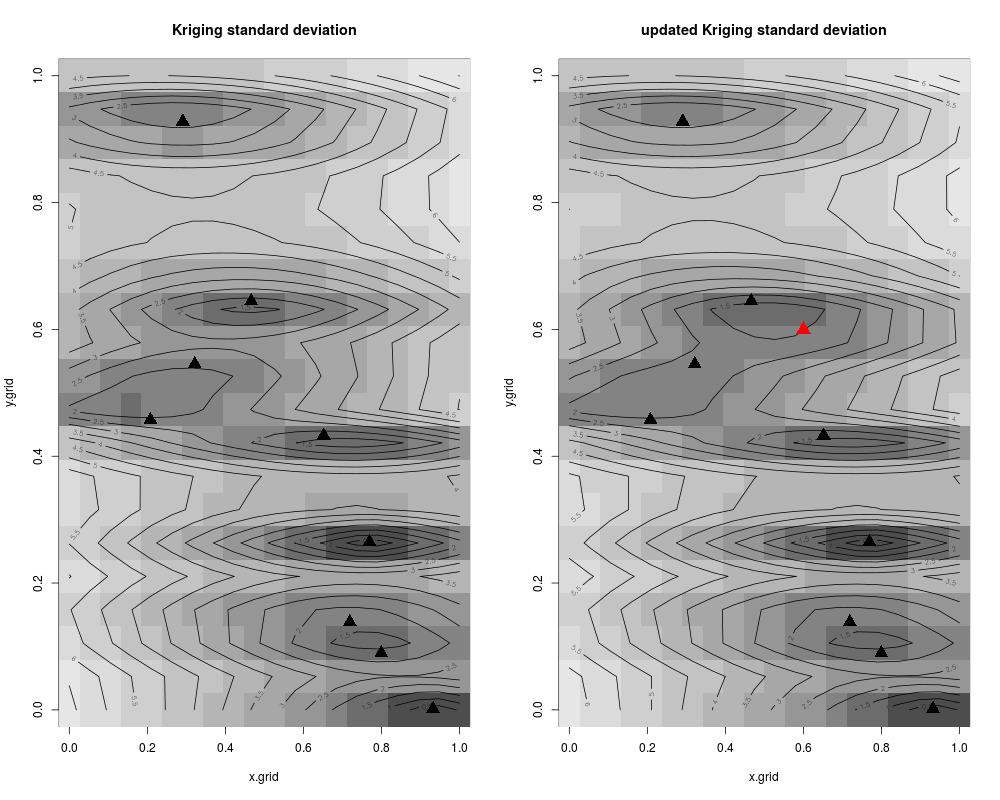
#the new kriging variance is usually lower than the old one
updated.predictions$sd - newdata.oldsd 

z.grid1 <- matrix(newdata.oldsd, n.grid, n.grid)
z.grid2 <- matrix(updated.predictions$sd, n.grid, n.grid)

par(mfrow=c(1,2))

#plots: contour of the criterion, doe points and new point
image(x=x.grid,y=y.grid,z=z.grid1,col=grey.colors(10))
contour(x=x.grid,y=y.grid,z=z.grid1,15,add=TRUE)
points(design, col="black", pch=17, lwd=4,cex=2)
title("Kriging standard deviation")

image(x=x.grid,y=y.grid,z=z.grid2,col=grey.colors(10))
contour(x=x.grid,y=y.grid,z=z.grid2,15,add=TRUE)
points(design, col="black", pch=17, lwd=4,cex=2)
points(new.x, col="red", pch=17, lwd=4,cex=2)
title("updated Kriging standard deviation")

Results

R version 3.3.1 (2016-06-21) -- "Bug in Your Hair"
Copyright (C) 2016 The R Foundation for Statistical Computing
Platform: x86_64-pc-linux-gnu (64-bit)

R is free software and comes with ABSOLUTELY NO WARRANTY.
You are welcome to redistribute it under certain conditions.
Type 'license()' or 'licence()' for distribution details.

R is a collaborative project with many contributors.
Type 'contributors()' for more information and
'citation()' on how to cite R or R packages in publications.

Type 'demo()' for some demos, 'help()' for on-line help, or
'help.start()' for an HTML browser interface to help.
Type 'q()' to quit R.

> library(KrigInv)
Loading required package: DiceKriging
Loading required package: pbivnorm
Loading required package: rgenoud
##  rgenoud (Version 5.7-12.4, Build Date: 2015-07-19)
##  See http://sekhon.berkeley.edu/rgenoud for additional documentation.
##  Please cite software as:
##   Walter Mebane, Jr. and Jasjeet S. Sekhon. 2011.
##   ``Genetic Optimization Using Derivatives: The rgenoud package for R.''
##   Journal of Statistical Software, 42(11): 1-26. 
##

Loading required package: randtoolbox
Loading required package: rngWELL
This is randtoolbox. For overview, type 'help("randtoolbox")'.
> png(filename="/home/ddbj/snapshot/RGM3/R_CC/result/KrigInv/predict_update_km.Rd_%03d_medium.png", width=480, height=480)
> ### Name: predict_update_km
> ### Title: Quick computation of updated kriging means and variances.
> ### Aliases: predict_update_km
> 
> ### ** Examples
> 
> #predict_update_km
> 
> set.seed(8)
> N <- 9 #number of observations
> testfun <- branin
> 
> #a 9 points initial design
> design <- data.frame( matrix(runif(2*N),ncol=2) )
> response <- testfun(design)
> 
> #km object with matern3_2 covariance
> #params estimated by ML from the observations
> model <- km(formula=~., design = design, 
+ 	response = response,covtype="matern3_2")

optimisation start
------------------
* estimation method   : MLE 
* optimisation method : BFGS 
* analytical gradient : used
* trend model : ~X1 + X2
* covariance model : 
  - type :  matern3_2 
  - nugget : NO
  - parameters lower bounds :  1e-10 1e-10 
  - parameters upper bounds :  1.448893 1.853021 
  - best initial criterion value(s) :  -25.38168 

N = 2, M = 5 machine precision = 2.22045e-16
At X0, 0 variables are exactly at the bounds
At iterate     0  f=       25.382  |proj g|=      0.19431
At iterate     1  f =       25.027  |proj g|=       0.13259
At iterate     2  f =       25.014  |proj g|=        1.6725
At iterate     3  f =       25.002  |proj g|=       0.15969
At iterate     4  f =       25.001  |proj g|=       0.17792
At iterate     5  f =       24.999  |proj g|=       0.31318
At iterate     6  f =       24.998  |proj g|=       0.14968
At iterate     7  f =       24.998  |proj g|=       0.03446
At iterate     8  f =       24.998  |proj g|=       0.03458
At iterate     9  f =       24.998  |proj g|=     0.0084816
At iterate    10  f =       24.998  |proj g|=      0.038393
At iterate    11  f =       24.997  |proj g|=        1.3196
At iterate    12  f =       24.997  |proj g|=        1.3327
At iterate    13  f =       24.994  |proj g|=        1.8077
At iterate    14  f =       24.991  |proj g|=        1.8106
At iterate    15  f =       24.975  |proj g|=        1.8136
At iterate    16  f =       24.937  |proj g|=        1.8202
At iterate    17  f =       24.816  |proj g|=        1.8136
At iterate    18  f =       24.652  |proj g|=       0.81261
At iterate    19  f =       24.652  |proj g|=       0.25743
At iterate    20  f =       24.651  |proj g|=     0.0033442
At iterate    21  f =       24.651  |proj g|=    1.4045e-05

iterations 21
function evaluations 30
segments explored during Cauchy searches 22
BFGS updates skipped 0
active bounds at final generalized Cauchy point 1
norm of the final projected gradient 1.40447e-05
final function value 24.6515

F = 24.6515
final  value 24.651471 
converged
> 
> #points where we want to compute prediction (if a point new.x is added to the doe)
> n.grid <- 20 #you can run it with 100
> x.grid <- y.grid <- seq(0,1,length=n.grid)
> newdata <- expand.grid(x.grid,y.grid)
> precalc.data <- precomputeUpdateData(model=model,integration.points=newdata)
> pred2 <- predict_nobias_km(object=model,newdata=newdata,type="UK",se.compute=TRUE)
> newdata.oldmean <- pred2$mean; newdata.oldsd <- pred2$sd
> 
> new.x <- matrix(c(0.6,0.6),ncol=2)   #the point that we are going to add
> pred1 <- predict_nobias_km(object=model,newdata=new.x,type="UK",se.compute=TRUE)
> newXmean <- pred1$mean; newXvar <- pred1$sd^2; newXvalue <- pred1$mean + 2*pred1$sd
> 
> kn <- computeQuickKrigcov(model=model,integration.points=newdata,X.new=new.x,
+                     precalc.data=precalc.data,F.newdata=pred1$F.newdata,
+                     c.newdata=pred1$c)
> 
> updated.predictions <- predict_update_km(newXmean=newXmean,newXvar=newXvar,
+ newXvalue=newXvalue,newdata.oldmean=newdata.oldmean,
+ newdata.oldsd=newdata.oldsd,kn=kn)
> 
> #the new kriging variance is usually lower than the old one
> updated.predictions$sd - newdata.oldsd 
  [1] -3.127812e-01 -2.939031e-01 -2.751519e-01 -2.565330e-01 -2.380516e-01
  [6] -2.197128e-01 -2.015210e-01 -1.834802e-01 -1.655938e-01 -1.478640e-01
 [11] -1.302921e-01 -1.128775e-01 -9.561736e-02 -7.850507e-02 -6.152702e-02
 [16] -4.465268e-02 -2.779693e-02 -1.059901e-02 -2.507032e-03 -2.005762e-02
 [21] -2.755457e-01 -2.552716e-01 -2.350283e-01 -2.148189e-01 -1.946493e-01
 [26] -1.745311e-01 -1.544852e-01 -1.345484e-01 -1.147842e-01 -9.529985e-02
 [31] -7.627278e-02 -5.798914e-02 -4.089384e-02 -2.564054e-02 -1.310754e-02
 [36] -4.318461e-03 -2.191451e-04 -1.348428e-03 -7.605062e-03 -1.830673e-02
 [41] -2.579623e-01 -2.382540e-01 -2.186423e-01 -1.991270e-01 -1.797063e-01
 [46] -1.603754e-01 -1.411265e-01 -1.219491e-01 -1.028332e-01 -8.377862e-02
 [51] -6.482553e-02 -4.614002e-02 -2.824675e-02 -1.256528e-02 -2.113892e-03
 [56] -6.809060e-04 -9.018736e-03 -2.379650e-02 -4.148245e-02 -6.023026e-02
 [61] -2.307591e-01 -2.105235e-01 -1.903588e-01 -1.702687e-01 -1.502603e-01
 [66] -1.303480e-01 -1.105630e-01 -9.097005e-02 -7.170215e-02 -5.302427e-02
 [71] -3.544490e-02 -1.987703e-02 -7.768630e-03 -9.404747e-04 -8.281939e-04
 [76] -7.492355e-03 -1.956469e-02 -3.520442e-02 -5.291099e-02 -7.173115e-02
 [81] -2.155749e-01 -1.948469e-01 -1.742464e-01 -1.538303e-01 -1.336784e-01
 [86] -1.139022e-01 -9.465491e-02 -7.614565e-02 -5.865414e-02 -4.254285e-02
 [91] -2.826137e-02 -1.633399e-02 -7.320645e-03 -1.746501e-03 -8.437985e-06
 [96] -2.284726e-03 -8.487893e-03 -1.828299e-02 -3.116906e-02 -4.657940e-02
[101] -2.485317e-01 -2.305172e-01 -2.126598e-01 -1.949637e-01 -1.774321e-01
[106] -1.600658e-01 -1.428596e-01 -1.258054e-01 -1.088936e-01 -9.211137e-02
[111] -7.544102e-02 -5.885622e-02 -4.231082e-02 -2.569365e-02 -8.569522e-03
[116] -4.299039e-03 -2.196496e-02 -3.945338e-02 -5.719797e-02 -7.529562e-02
[121] -1.919058e-01 -1.720945e-01 -1.525328e-01 -1.332971e-01 -1.144881e-01
[126] -9.623331e-02 -7.868425e-02 -6.204195e-02 -4.657142e-02 -3.260705e-02
[131] -2.055130e-02 -1.086031e-02 -4.010045e-03 -4.419493e-04 -4.920985e-04
[136] -4.309904e-03 -1.181502e-02 -2.271150e-02 -3.655515e-02 -5.283641e-02
[141] -1.737945e-01 -1.551295e-01 -1.368969e-01 -1.191866e-01 -1.021064e-01
[146] -8.576704e-02 -7.024916e-02 -5.566315e-02 -4.217351e-02 -3.000027e-02
[151] -1.942078e-02 -1.076748e-02 -4.415293e-03 -7.571034e-04 -1.606447e-04
[156] -2.870925e-03 -8.953997e-03 -1.829306e-02 -3.061887e-02 -4.556119e-02
[161] -1.679841e-01 -1.527740e-01 -1.381727e-01 -1.242276e-01 -1.109901e-01
[166] -9.846163e-02 -8.645812e-02 -7.475646e-02 -6.315645e-02 -5.146150e-02
[171] -3.949911e-02 -2.724011e-02 -1.515498e-02 -4.983101e-03 -8.812585e-05
[176] -2.852639e-03 -1.236140e-02 -2.616131e-02 -4.238107e-02 -6.002621e-02
[181] -3.695395e-02 -2.016739e-02 -7.477629e-03 -8.089445e-04 -7.522605e-04
[186] -5.979475e-03 -1.452867e-02 -2.499077e-02 -3.657534e-02 -4.889596e-02
[191] -6.178906e-02 -7.518951e-02 -8.908311e-02 -1.035339e-01 -1.185621e-01
[196] -1.341181e-01 -1.501581e-01 -1.666436e-01 -1.835403e-01 -2.008172e-01
[201] -1.886952e-01 -1.624269e-01 -1.340818e-01 -1.037956e-01 -7.273489e-02
[206] -4.358868e-02 -2.004385e-02 -5.194533e-03 -2.153522e-05 -3.372126e-03
[211] -1.325637e-02 -2.772119e-02 -4.514132e-02 -6.440053e-02 -8.482674e-02
[216] -1.059776e-01 -1.275683e-01 -1.494147e-01 -1.713973e-01 -1.934388e-01
[221] -5.818834e-02 -9.919695e-02 -1.558252e-01 -2.312517e-01 -3.286174e-01
[226] -4.502402e-01 -5.962980e-01 -7.627823e-01 -9.397185e-01 -1.111499e+00
[231] -1.259998e+00 -1.370277e+00 -1.436567e+00 -1.465246e+00 -1.468181e+00
[236] -1.455351e+00 -1.433667e+00 -1.407506e+00 -1.379528e+00 -1.351319e+00
[241] -3.113054e-02 -1.725866e-02 -6.608816e-03 -6.220008e-04 -1.550415e-03
[246] -1.295480e-02 -4.034805e-02 -9.128997e-02 -1.720636e-01 -2.767965e-01
[251] -3.790648e-01 -4.536553e-01 -4.987397e-01 -5.253226e-01 -5.428750e-01
[256] -5.562937e-01 -5.678378e-01 -5.785354e-01 -5.888648e-01 -5.990574e-01
[261] -2.340407e-01 -2.112460e-01 -1.874163e-01 -1.626197e-01 -1.370758e-01
[266] -1.112183e-01 -8.574464e-02 -6.162789e-02 -4.005485e-02 -2.224615e-02
[271] -9.285912e-03 -1.880338e-03 -7.081184e-05 -3.377521e-03 -1.110483e-02
[276] -2.252006e-02 -3.693900e-02 -5.376640e-02 -7.250628e-02 -9.275595e-02
[281] -8.420206e-02 -6.689303e-02 -5.086093e-02 -3.642994e-02 -2.394730e-02
[286] -1.376309e-02 -6.204617e-03 -1.549430e-03 -3.695647e-07 -1.667388e-03
[291] -6.555684e-03 -1.453596e-02 -2.535428e-02 -3.869219e-02 -5.421641e-02
[296] -7.159602e-02 -9.051982e-02 -1.107071e-01 -1.319122e-01 -1.539258e-01
[301] -4.046043e-02 -2.793468e-02 -1.740282e-02 -9.143648e-03 -3.412879e-03
[306] -4.216175e-04 -3.160843e-04 -3.162024e-03 -8.936513e-03 -1.753124e-02
[311] -2.876152e-02 -4.237281e-02 -5.806730e-02 -7.553752e-02 -9.448870e-02
[316] -1.146479e-01 -1.357720e-01 -1.576508e-01 -1.801070e-01 -2.029944e-01
[321] -3.113182e-02 -1.993492e-02 -1.095443e-02 -4.491813e-03 -8.116494e-04
[326] -1.133694e-04 -2.506233e-03 -7.991484e-03 -1.645716e-02 -2.769311e-02
[331] -4.141649e-02 -5.729930e-02 -7.499956e-02 -9.418842e-02 -1.145672e-01
[336] -1.358749e-01 -1.578911e-01 -1.804345e-01 -2.033591e-01 -2.265495e-01
[341] -4.969946e-02 -3.457481e-02 -2.132093e-02 -1.064210e-02 -3.325351e-03
[346] -1.038513e-04 -1.463269e-03 -7.469523e-03 -1.773420e-02 -3.156161e-02
[351] -4.815538e-02 -6.677771e-02 -8.682825e-02 -1.078581e-01 -1.295493e-01
[356] -1.516835e-01 -1.741136e-01 -1.967409e-01 -2.194993e-01 -2.423439e-01
[361] -5.295223e-02 -3.679766e-02 -2.217700e-02 -1.017625e-02 -2.290770e-03
[366] -7.650683e-05 -4.390055e-03 -1.477538e-02 -2.975726e-02 -4.770488e-02
[371] -6.737985e-02 -8.801350e-02 -1.091796e-01 -1.306559e-01 -1.523301e-01
[376] -1.741459e-01 -1.960743e-01 -2.180992e-01 -2.402104e-01 -2.623999e-01
[381] -8.411805e-03 -3.001644e-03 -2.896661e-04 -4.547391e-04 -3.592728e-03
[386] -9.701084e-03 -1.867504e-02 -3.031400e-02 -4.434248e-02 -6.044333e-02
[391] -7.828790e-02 -9.755996e-02 -1.179718e-01 -1.392728e-01 -1.612520e-01
[396] -1.837367e-01 -2.065882e-01 -2.296972e-01 -2.529789e-01 -2.763681e-01
> 
> z.grid1 <- matrix(newdata.oldsd, n.grid, n.grid)
> z.grid2 <- matrix(updated.predictions$sd, n.grid, n.grid)
> 
> par(mfrow=c(1,2))
> 
> #plots: contour of the criterion, doe points and new point
> image(x=x.grid,y=y.grid,z=z.grid1,col=grey.colors(10))
> contour(x=x.grid,y=y.grid,z=z.grid1,15,add=TRUE)
> points(design, col="black", pch=17, lwd=4,cex=2)
> title("Kriging standard deviation")
> 
> image(x=x.grid,y=y.grid,z=z.grid2,col=grey.colors(10))
> contour(x=x.grid,y=y.grid,z=z.grid2,15,add=TRUE)
> points(design, col="black", pch=17, lwd=4,cex=2)
> points(new.x, col="red", pch=17, lwd=4,cex=2)
> title("updated Kriging standard deviation")
> 
> 
> 
> 
> 
> 
> dev.off()
null device 
          1 
>