Supported by Dr. Osamu Ogasawara and  . . |
|
Last data update: 2014.03.03 |
Quick update of kriging means and variances when many new points are added.DescriptionThis function is the parallel version of the function Usagepredict_update_km_parallel(newXmean, newXvar, newXvalue, Sigma.r, newdata.oldmean, newdata.oldsd, kn) Arguments
ValueA list with the following fields:
Author(s)Clement Chevalier (IMSV, Switzerland, and IRSN, France) ReferencesChevalier C., Bect J., Ginsbourger D., Vazquez E., Picheny V., Richet Y. (2011), Fast parallel kriging-based stepwise uncertainty reduction with application to the identification of an excursion set ,http://hal.archives-ouvertes.fr/hal-00641108/ Chevalier C., Ginsbourger D. (2012), Corrected Kriging update formulae for batch-sequential data assimilation ,http://arxiv.org/pdf/1203.6452.pdf See Also
Examples
#predict_update_km_parallel
set.seed(8)
N <- 9 #number of observations
testfun <- branin
#a 9 points initial design
design <- data.frame( matrix(runif(2*N),ncol=2) )
response <- testfun(design)
#km object with matern3_2 covariance
#params estimated by ML from the observations
model <- km(formula=~., design = design,
response = response,covtype="matern3_2")
#points where we want to compute prediction (if a point new.x is added to the doe)
n.grid <- 20 #you can run it with 100
x.grid <- y.grid <- seq(0,1,length=n.grid)
newdata <- expand.grid(x.grid,y.grid)
precalc.data <- precomputeUpdateData(model=model,integration.points=newdata)
pred2 <- predict_nobias_km(object=model,newdata=newdata,type="UK",se.compute=TRUE)
newdata.oldmean <- pred2$mean; newdata.oldsd <- pred2$sd
#the point that we are going to add
new.x <- matrix(c(0.1,0.2,0.3,0.4,0.5,0.6,0.7,0.8),ncol=2,byrow=TRUE)
pred1 <- predict_nobias_km(object=model,newdata=new.x,type="UK",
se.compute=TRUE,cov.compute=TRUE)
newXmean <- pred1$mean; newXvar <- pred1$sd^2; newXvalue <- pred1$mean + 2*pred1$sd
Sigma.r <- pred1$cov
kn <- computeQuickKrigcov(model=model,integration.points=newdata,X.new=new.x,
precalc.data=precalc.data,F.newdata=pred1$F.newdata,
c.newdata=pred1$c)
updated.predictions <- predict_update_km_parallel(newXmean=newXmean,newXvar=newXvar,
newXvalue=newXvalue,Sigma.r=Sigma.r,
newdata.oldmean=newdata.oldmean,
newdata.oldsd=newdata.oldsd,kn=kn)
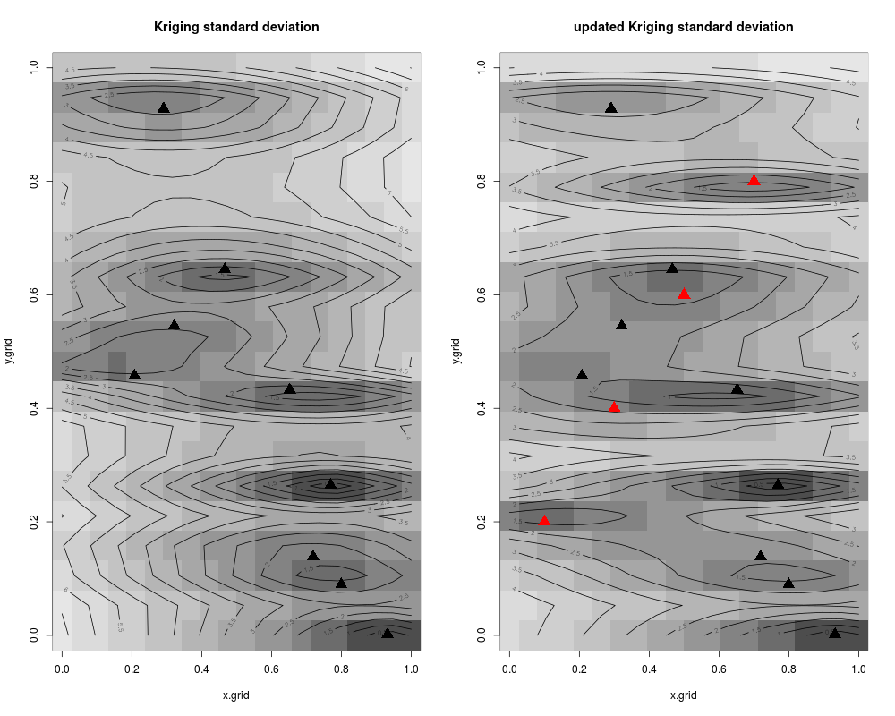
#the new kriging variance is usually lower than the old one
updated.predictions$sd - newdata.oldsd
z.grid1 <- matrix(newdata.oldsd, n.grid, n.grid)
z.grid2 <- matrix(updated.predictions$sd, n.grid, n.grid)
par(mfrow=c(1,2))
#plots: contour of the criterion, doe points and new point
image(x=x.grid,y=y.grid,z=z.grid1,col=grey.colors(10))
contour(x=x.grid,y=y.grid,z=z.grid1,15,add=TRUE)
points(design, col="black", pch=17, lwd=4,cex=2)
title("Kriging standard deviation")
image(x=x.grid,y=y.grid,z=z.grid2,col=grey.colors(10))
contour(x=x.grid,y=y.grid,z=z.grid2,15,add=TRUE)
points(design, col="black", pch=17, lwd=4,cex=2)
points(new.x, col="red", pch=17, lwd=4,cex=2)
title("updated Kriging standard deviation")
Results
R version 3.3.1 (2016-06-21) -- "Bug in Your Hair"
Copyright (C) 2016 The R Foundation for Statistical Computing
Platform: x86_64-pc-linux-gnu (64-bit)

R is free software and comes with ABSOLUTELY NO WARRANTY.
You are welcome to redistribute it under certain conditions.
Type 'license()' or 'licence()' for distribution details.

R is a collaborative project with many contributors.
Type 'contributors()' for more information and
'citation()' on how to cite R or R packages in publications.

Type 'demo()' for some demos, 'help()' for on-line help, or
'help.start()' for an HTML browser interface to help.
Type 'q()' to quit R.

> library(KrigInv)
Loading required package: DiceKriging
Loading required package: pbivnorm
Loading required package: rgenoud
##  rgenoud (Version 5.7-12.4, Build Date: 2015-07-19)
##  See http://sekhon.berkeley.edu/rgenoud for additional documentation.
##  Please cite software as:
##   Walter Mebane, Jr. and Jasjeet S. Sekhon. 2011.
##   ``Genetic Optimization Using Derivatives: The rgenoud package for R.''
##   Journal of Statistical Software, 42(11): 1-26.
##

Loading required package: randtoolbox
Loading required package: rngWELL
This is randtoolbox. For overview, type 'help("randtoolbox")'.
> png(filename="/home/ddbj/snapshot/RGM3/R_CC/result/KrigInv/predict_update_km_parallel.Rd_%03d_medium.png", width=480, height=480)
> ### Name: predict_update_km_parallel
> ### Title: Quick update of kriging means and variances when many new points
> ###   are added.
> ### Aliases: predict_update_km_parallel
>
> ### ** Examples
>
> #predict_update_km_parallel
>
> set.seed(8)
> N <- 9 #number of observations
> testfun <- branin
>
> #a 9 points initial design
> design <- data.frame( matrix(runif(2*N),ncol=2) )
> response <- testfun(design)
>
> #km object with matern3_2 covariance
> #params estimated by ML from the observations
> model <- km(formula=~., design = design,
+ 	response = response,covtype="matern3_2")

optimisation start
------------------
* estimation method   : MLE
* optimisation method : BFGS
* analytical gradient : used
* trend model : ~X1 + X2
* covariance model :
  - type :  matern3_2
  - nugget : NO
  - parameters lower bounds :  1e-10 1e-10
  - parameters upper bounds :  1.448893 1.853021
  - best initial criterion value(s) :  -25.38168

N = 2, M = 5 machine precision = 2.22045e-16
At X0, 0 variables are exactly at the bounds
At iterate     0  f=       25.382  |proj g|=      0.19431
At iterate     1  f =       25.027  |proj g|=       0.13259
At iterate     2  f =       25.014  |proj g|=        1.6725
At iterate     3  f =       25.002  |proj g|=       0.15969
At iterate     4  f =       25.001  |proj g|=       0.17792
At iterate     5  f =       24.999  |proj g|=       0.31318
At iterate     6  f =       24.998  |proj g|=       0.14968
At iterate     7  f =       24.998  |proj g|=       0.03446
At iterate     8  f =       24.998  |proj g|=       0.03458
At iterate     9  f =       24.998  |proj g|=     0.0084816
At iterate    10  f =       24.998  |proj g|=      0.038393
At iterate    11  f =       24.997  |proj g|=        1.3196
At iterate    12  f =       24.997  |proj g|=        1.3327
At iterate    13  f =       24.994  |proj g|=        1.8077
At iterate    14  f =       24.991  |proj g|=        1.8106
At iterate    15  f =       24.975  |proj g|=        1.8136
At iterate    16  f =       24.937  |proj g|=        1.8202
At iterate    17  f =       24.816  |proj g|=        1.8136
At iterate    18  f =       24.652  |proj g|=       0.81261
At iterate    19  f =       24.652  |proj g|=       0.25743
At iterate    20  f =       24.651  |proj g|=     0.0033442
At iterate    21  f =       24.651  |proj g|=    1.4045e-05

iterations 21
function evaluations 30
segments explored during Cauchy searches 22
BFGS updates skipped 0
active bounds at final generalized Cauchy point 1
norm of the final projected gradient 1.40447e-05
final function value 24.6515

F = 24.6515
final  value 24.651471
converged
>
> #points where we want to compute prediction (if a point new.x is added to the doe)
> n.grid <- 20 #you can run it with 100
> x.grid <- y.grid <- seq(0,1,length=n.grid)
> newdata <- expand.grid(x.grid,y.grid)
> precalc.data <- precomputeUpdateData(model=model,integration.points=newdata)
> pred2 <- predict_nobias_km(object=model,newdata=newdata,type="UK",se.compute=TRUE)
> newdata.oldmean <- pred2$mean; newdata.oldsd <- pred2$sd
>
> #the point that we are going to add
> new.x <- matrix(c(0.1,0.2,0.3,0.4,0.5,0.6,0.7,0.8),ncol=2,byrow=TRUE)
> pred1 <- predict_nobias_km(object=model,newdata=new.x,type="UK",
+ se.compute=TRUE,cov.compute=TRUE)
> newXmean <- pred1$mean; newXvar <- pred1$sd^2; newXvalue <- pred1$mean + 2*pred1$sd
> Sigma.r <- pred1$cov
>
> kn <- computeQuickKrigcov(model=model,integration.points=newdata,X.new=new.x,
+                     precalc.data=precalc.data,F.newdata=pred1$F.newdata,
+                     c.newdata=pred1$c)
>
> updated.predictions <- predict_update_km_parallel(newXmean=newXmean,newXvar=newXvar,
+                                          newXvalue=newXvalue,Sigma.r=Sigma.r,
+                                          newdata.oldmean=newdata.oldmean,
+                                          newdata.oldsd=newdata.oldsd,kn=kn)
>
> #the new kriging variance is usually lower than the old one
> updated.predictions$sd - newdata.oldsd
  [1] -2.323265383 -2.174667611 -2.027531617 -1.881969295 -1.738111333
  [6] -1.596090849 -1.456039142 -1.318084796 -1.182352546 -1.048961742
 [11] -0.918024281 -0.789641469 -0.663898556 -0.540853715 -0.420511002
 [16] -0.302715262 -0.186829284 -0.070100610 -0.014000257 -0.126767948
 [21] -2.074913534 -1.914509823 -1.754723370 -1.595719371 -1.437773584
 [26] -1.281232185 -1.126530213 -0.974239033 -0.825136199 -0.680305760
 [31] -0.541276564 -0.410197629 -0.290026157 -0.184653076 -0.098811324
 [36] -0.037530569 -0.005122898 -0.003874074 -0.033102747 -0.089419149
 [41] -1.959588166 -1.798603189 -1.637970295 -1.477850304 -1.318680496
 [46] -1.160937320 -1.005096635 -0.851663721 -0.701238097 -0.554655265
 [51] -0.413304415 -0.279832969 -0.159626285 -0.063343909 -0.008624105
 [56] -0.013182685 -0.077228904 -0.180772314 -0.302606971 -0.430607467
 [61] -2.669003954 -2.493378910 -2.309983918 -2.118150579 -1.918857319
 [66] -1.713406574 -1.503170170 -1.289727954 -1.075149924 -0.862504470
 [71] -0.656658936 -0.465257123 -0.299254412 -0.171634975 -0.093142541
 [76] -0.066834695 -0.086824410 -0.142648020 -0.223943514 -0.322588999
 [81] -4.748195470 -4.587123280 -4.368832868 -4.085877137 -3.751183354
 [86] -3.385170399 -3.006436340 -2.629016820 -2.262983300 -1.915800384
 [91] -1.593380397 -1.300679233 -1.041904588 -0.820435013 -0.638565934
 [96] -0.497111543 -0.395210438 -0.330577455 -0.299908210 -0.299346107
[101] -2.200085288 -2.046015679 -1.890233382 -1.732754661 -1.574312426
[106] -1.415719185 -1.257700074 -1.100950293 -0.946159652 -0.793938822
[111] -0.644799004 -0.499117320 -0.357023590 -0.217900701 -0.077198506
[116] -0.024814638 -0.152068708 -0.280719616 -0.409028838 -0.537749386
[121] -1.741239517 -1.582938652 -1.425467136 -1.269461332 -1.115821971
[126] -0.965618142 -0.820045415 -0.680747523 -0.549957006 -0.430164138
[131] -0.324043385 -0.234357702 -0.163791938 -0.114712532 -0.088839077
[136] -0.086930797 -0.108677103 -0.152793874 -0.217241158 -0.299537432
[141] -2.801807557 -2.668393100 -2.527867813 -2.379138329 -2.221392819
[146] -2.054142706 -1.877125561 -1.692202740 -1.504137460 -1.317957638
[151] -1.138536488 -0.970490644 -0.818110437 -0.685269259 -0.575093844
[156] -0.489724770 -0.430300792 -0.396954297 -0.388900763 -0.404638698
[161] -2.136982935 -2.030269766 -1.923271367 -1.814840914 -1.703488403
[166] -1.587123191 -1.462390978 -1.327156865 -1.182139293 -1.027408521
[171] -0.861737590 -0.683670788 -0.496461585 -0.317657922 -0.181238649
[176] -0.111793001 -0.107188911 -0.150775985 -0.226467018 -0.323272155
[181] -0.150340545 -0.063397255 -0.013136779 -0.006923464 -0.042826380
[186] -0.109372774 -0.193791038 -0.287417944 -0.385593073 -0.486234864
[191] -0.588561637 -0.692348472 -0.797569099 -0.904230722 -1.012232286
[196] -1.121471453 -1.231927683 -1.343628012 -1.456619881 -1.570955139
[201] -0.482198698 -0.357241372 -0.244746709 -0.150491241 -0.082032877
[206] -0.046880860 -0.049010162 -0.086275444 -0.151539909 -0.236379835
[211] -0.333923332 -0.439494635 -0.550237485 -0.664568930 -0.781570257
[216] -0.900689676 -1.021623412 -1.144204888 -1.268340006 -1.393970998
[221] -1.101535807 -1.037882950 -0.989967460 -0.960197958 -0.950734191
[226] -0.962785074 -0.995638054 -1.045802861 -1.106922938 -1.171350650
[231] -1.232299883 -1.287996762 -1.341561295 -1.396288758 -1.454608213
[236] -1.517976393 -1.587103621 -1.662208956 -1.743220061 -1.829905680
[241] -0.990435495 -0.873677455 -0.761178520 -0.653967545 -0.553666852
[246] -0.462926697 -0.386141926 -0.330335823 -0.304687584 -0.316115263
[251] -0.362061557 -0.433022196 -0.520367274 -0.618484561 -0.724217183
[256] -0.835779105 -0.952095648 -1.072464848 -1.196391503 -1.323501468
[261] -0.685576457 -0.571077419 -0.464891113 -0.369024101 -0.285857133
[266] -0.218074251 -0.168480714 -0.139697377 -0.133748868 -0.151623252
[271] -0.193041041 -0.256448752 -0.339229934 -0.438300720 -0.550559376
[276] -0.673255106 -0.804101628 -0.941253260 -1.083264242 -1.229023622
[281] -0.690671420 -0.628165221 -0.579134535 -0.544852611 -0.526462509
[286] -0.524881139 -0.540699671 -0.574088941 -0.624734044 -0.691818593
[291] -0.774038239 -0.869637362 -0.976544523 -1.092515334 -1.215310701
[296] -1.343333157 -1.475481180 -1.610836194 -1.748653005 -1.888343623
[301] -1.560270720 -1.618009211 -1.699447804 -1.806039775 -1.938894251
[306] -2.098600430 -2.285004499 -2.496873758 -2.731471440 -2.983981003
[311] -3.246566269 -3.507107438 -3.748296240 -3.949194330 -4.092741615
[316] -4.180753473 -4.228850539 -4.253379430 -4.266654595 -4.276651080
[321] -0.827939155 -0.811314230 -0.811687866 -0.830123147 -0.867350424
[326] -0.923643820 -0.998711273 -1.091534209 -1.200337469 -1.322745041
[331] -1.455909461 -1.596671044 -1.741743773 -1.887892672 -2.032217250
[336] -2.173469132 -2.311539913 -2.446607273 -2.579026612 -2.709247873
[341] -0.374561866 -0.282644355 -0.205053087 -0.145568502 -0.108163706
[346] -0.096378800 -0.112505100 -0.156781211 -0.227226310 -0.320324090
[351] -0.431883606 -0.557765006 -0.694313726 -0.838521112 -0.988027216
[356] -1.141190596 -1.296910931 -1.454415463 -1.613164959 -1.772784110
[361] -0.354756653 -0.247380633 -0.151720131 -0.074044361 -0.022401864
[366] -0.004867445 -0.026163671 -0.084800986 -0.173947666 -0.285129715
[371] -0.411068783 -0.546586856 -0.688354233 -0.834329470 -0.983277123
[376] -1.134466762 -1.287461767 -1.441982190 -1.597835472 -1.754877643
[381] -0.179615438 -0.141560879 -0.119446797 -0.114231569 -0.126538583
[386] -0.156588056 -0.204162484 -0.268556900 -0.348631292 -0.442979393
[391] -0.550048419 -0.668243374 -0.796009584 -0.931890324 -1.074562258
[396] -1.222860365 -1.375776854 -1.532448486 -1.692144053 -1.854249557
>
> z.grid1 <- matrix(newdata.oldsd, n.grid, n.grid)
> z.grid2 <- matrix(updated.predictions$sd, n.grid, n.grid)
>
> par(mfrow=c(1,2))
>
> #plots: contour of the criterion, doe points and new point
> image(x=x.grid,y=y.grid,z=z.grid1,col=grey.colors(10))
> contour(x=x.grid,y=y.grid,z=z.grid1,15,add=TRUE)
> points(design, col="black", pch=17, lwd=4,cex=2)
> title("Kriging standard deviation")
>
> image(x=x.grid,y=y.grid,z=z.grid2,col=grey.colors(10))
> contour(x=x.grid,y=y.grid,z=z.grid2,15,add=TRUE)
> points(design, col="black", pch=17, lwd=4,cex=2)
> points(new.x, col="red", pch=17, lwd=4,cex=2)
> title("updated Kriging standard deviation")
>
>
>
>
>
> dev.off()
null device
          1
>
|