R Graphical Manual

Browse All

Last data update: 2014.03.03

R: Prints a measure of uncertainty for 1d function.

print_uncertainty_1d

R Documentation

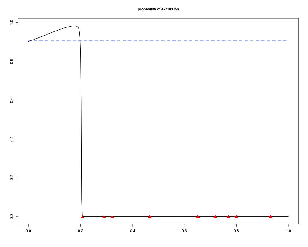
Prints a measure of uncertainty for 1d function.

Description

This function draws the value of a given measure of uncertainty over the whole input domain (1D). Possible measures are "pn" (beeing the probability of excursion) and measures specific to a sampling criterion: "sur", "timse" and "imse". This function can be used to print relevant outputs after having used the function EGI.

Usage

print_uncertainty_1d(model, T, type = "pn", 
lower = 0, upper = 1, resolution = 500, 
new.points = 0, xlab = "", ylab = "", main = "", 
xscale = c(0, 1), show.points = TRUE, cex.main = 1, cex.lab = 1, 
cex.points = 1, cex.axis = 1, pch.points.init = 17, pch.points.end = 17, 
col.points.init = "black", col.points.end = "red", xaxislab = NULL, 
yaxislab = NULL, xaxispoint = NULL, yaxispoint = NULL, 
xdecal = 3, ydecal = 3,DiceViewplot=FALSE,vorobmean=FALSE)

Arguments

`model`	Kriging model of `km` class.
`T`	Target value (scalar).
`type`	Type of uncertainty that the user wants to print. Possible values are `"pn"` (probability of excursion), or `"sur"`, `"imse"`, `"timse"`, `"vorob"` if we print a measure of uncertainty corresponding to one criterion.
`lower`	Lower bound for the input domain.
`upper`	Upper bound for the input domain.
`resolution`	Number of points to discretize the interval (lower,upper).
`new.points`	Number of new observations. These observations are the last new.points observations and can be printed in another color and the initial observations (see argument: `col.points.end`).
`xlab`	Label for the x axis.
`ylab`	Label for the y axis.
`main`	Title of the graph.
`xscale`	If one wants to rescale the input domain on another interval it is possible to set this vector of size 2. The new interval will be translated by `xscale[1]` and expanded by a factor `xscale[2] - xscale[1]`.
`show.points`	Boolean: should we show the observations on the graph ?
`cex.main`	Multiplicative factor for the size of the title.
`cex.lab`	Multiplicative factor for the size of titles of the axis.
`cex.points`	Multiplicative factor for the size of the points.
`cex.axis`	Multiplicative factor for the size of the axis graduations.
`pch.points.init`	Symbol for the `n-new.points` first observations.
`pch.points.end`	Symbol for the `new.points` last observations.
`col.points.init`	Color for the `n-new.points` first observations.
`col.points.end`	Color for the `new.points` last observations.
`xaxislab`	Optional new labels that will replace the normal levels on x axis.
`yaxislab`	Optional new labels that will replace the normal levels on y axis.
`xaxispoint`	Position of these new labels on x axis.
`yaxispoint`	Position of these new labels on y axis.
`xdecal`	Optional position shifting of the titles of the x axis.
`ydecal`	Optional position shifting of the titles of the y axis.
`DiceViewplot`	Optional boolean. When it is set to `TRUE` (default) a second plot is added, generated with the DiceView package. This plot shows the kriging mean and confidence intervals on the whole input domain.
`vorobmean`	Optional boolean. When it is set to `TRUE` the Vorob'ev expectation is plotted. It corresponds to the averaged excursion set, using the definition of Vorob'ev. Here, the estimated set is the set above the Vorob'ev threshold (plotted in blue).

Value

the integrated uncertainty

Author(s)

Clement Chevalier (IMSV, Switzerland, and IRSN, France)

References

Bect J., Ginsbourger D., Li L., Picheny V., Vazquez E. (2010), Sequential design of computer experiments for the estimation of a probability of failure, Statistics and Computing, pp.1-21, 2011, http://arxiv.org/abs/1009.5177

Examples

#print_uncertainty_1d

set.seed(8)
N <- 9 #number of observations
T <- 1 #threshold
testfun <- fundet
lower <- c(0)
upper <- c(1)

#a 9 points initial design
design <- data.frame( matrix(runif(N),ncol=1) )
response <- testfun(design)

#km object with matern3_2 covariance
#params estimated by ML from the observations
model <- km(formula=~., design = design, 
	response = response,covtype="matern3_2")

print_uncertainty_1d(DiceViewplot=FALSE,model=model,T=T,
main="probability of excursion",cex.points=1.5,col.points.init="red",vorobmean=TRUE)

Results


R version 3.3.1 (2016-06-21) -- "Bug in Your Hair"
Copyright (C) 2016 The R Foundation for Statistical Computing
Platform: x86_64-pc-linux-gnu (64-bit)

R is free software and comes with ABSOLUTELY NO WARRANTY.
You are welcome to redistribute it under certain conditions.
Type 'license()' or 'licence()' for distribution details.

R is a collaborative project with many contributors.
Type 'contributors()' for more information and
'citation()' on how to cite R or R packages in publications.

Type 'demo()' for some demos, 'help()' for on-line help, or
'help.start()' for an HTML browser interface to help.
Type 'q()' to quit R.

> library(KrigInv)
Loading required package: DiceKriging
Loading required package: pbivnorm
Loading required package: rgenoud
##  rgenoud (Version 5.7-12.4, Build Date: 2015-07-19)
##  See http://sekhon.berkeley.edu/rgenoud for additional documentation.
##  Please cite software as:
##   Walter Mebane, Jr. and Jasjeet S. Sekhon. 2011.
##   ``Genetic Optimization Using Derivatives: The rgenoud package for R.''
##   Journal of Statistical Software, 42(11): 1-26. 
##

Loading required package: randtoolbox
Loading required package: rngWELL
This is randtoolbox. For overview, type 'help("randtoolbox")'.
> png(filename="/home/ddbj/snapshot/RGM3/R_CC/result/KrigInv/print_uncertainty_1d.Rd_%03d_medium.png", width=480, height=480)
> ### Name: print_uncertainty_1d
> ### Title: Prints a measure of uncertainty for 1d function.
> ### Aliases: print_uncertainty_1d
> 
> ### ** Examples
> 
> #print_uncertainty_1d
> 
> set.seed(8)
> N <- 9 #number of observations
> T <- 1 #threshold
> testfun <- fundet
> lower <- c(0)
> upper <- c(1)
> 
> #a 9 points initial design
> design <- data.frame( matrix(runif(N),ncol=1) )
> response <- testfun(design)
> 
> #km object with matern3_2 covariance
> #params estimated by ML from the observations
> model <- km(formula=~., design = design, 
+ 	response = response,covtype="matern3_2")

optimisation start
------------------
* estimation method   : MLE 
* optimisation method : BFGS 
* analytical gradient : used
* trend model : ~matrix.runif.N...ncol...1.
* covariance model : 
  - type :  matern3_2 
  - nugget : NO
  - parameters lower bounds :  1e-10 
  - parameters upper bounds :  1.448893 
  - best initial criterion value(s) :  6.967818 

N = 1, M = 5 machine precision = 2.22045e-16
At X0, 0 variables are exactly at the bounds
At iterate     0  f=      -6.9678  |proj g|=      0.71529
At iterate     1  f =      -6.9717  |proj g|=       0.46395
At iterate     2  f =       -6.979  |proj g|=      0.077446
At iterate     3  f =      -6.9792  |proj g|=      0.010775
At iterate     4  f =      -6.9792  |proj g|=     0.0002012
At iterate     5  f =      -6.9792  |proj g|=    5.0988e-07

iterations 5
function evaluations 7
segments explored during Cauchy searches 5
BFGS updates skipped 0
active bounds at final generalized Cauchy point 0
norm of the final projected gradient 5.09875e-07
final function value -6.97921

F = -6.97921
final  value -6.979214 
converged
> 
> print_uncertainty_1d(DiceViewplot=FALSE,model=model,T=T,
+ main="probability of excursion",cex.points=1.5,col.points.init="red",vorobmean=TRUE)
[1] 0.1927658
> 
> 
> 
> 
> 
> 
> 
> dev.off()
null device 
          1 
>