R Graphical Manual

Browse All

Last data update: 2014.03.03

R: Parallel timse criterion

timse_optim_parallel2

R Documentation

Parallel timse criterion

Description

Evaluation of the parallel timse criterion for some candidate points, assuming that some other points are also going to be evaluated. To be used in optimization routines, like in max_timse_parallel. To avoid numerical instabilities, the new points are evaluated only if they are not too close to an existing observation, or if there is some observation noise. The criterion is the integral of the posterior timse uncertainty.

Usage

timse_optim_parallel2(x, other.points, 
integration.points, integration.weights = NULL, 
intpoints.oldmean, intpoints.oldsd, precalc.data, 
model, T, new.noise.var = NULL,weight = NULL, 
batchsize, current.timse)

Arguments

`x`	Input vector of size d at which one wants to evaluate the criterion. This argument corresponds to only ONE point.
`other.points`	Vector giving the other `batchsize-1` points at which one wants to evaluate the criterion
`integration.points`	p*d matrix of points for numerical integration in the X space.
`integration.weights`	Vector of size p corresponding to the weights of these integration points.
`intpoints.oldmean`	Vector of size p corresponding to the kriging mean at the integration points before adding `x` to the design of experiments.
`intpoints.oldsd`	Vector of size p corresponding to the kriging standard deviation at the integration points before adding `x` to the design of experiments.
`precalc.data`	List containing useful data to compute quickly the updated kriging variance. This list can be generated using the `precomputeUpdateData` function.
`model`	Object of class `km` (Kriging model).
`T`	Target value (scalar).
`new.noise.var`	Optional scalar value of the noise variance for the new observations.
`weight`	Vector of weight function (length must be equal to the number of lines of the matrix integration.points). If nothing is set, the imse criterion is used instead of timse. It corresponds to equal weights.
`batchsize`	Number of points to sample simultaneously. The sampling criterion will return batchsize points at a time for sampling.
`current.timse`	Current value of the timse criterion (before adding new observations)

Details

The first argument x has been chosen to be a vector of size d so that an optimizer like genoud can optimize it easily. The second argument other.points is a vector of size (batchsize-1)*d corresponding to the batchsize-1 other points. The last argument current.timse is used as a default value for the timse criterion when the new points x are too close to existing observations.

Value

Parallel timse value

Author(s)

Victor Picheny (CERFACS, Toulouse, France)

Clement Chevalier (IMSV, Switzerland, and IRSN, France)

References

Picheny, V., Ginsbourger, D., Roustant, O., Haftka, R.T., Adaptive designs of experiments for accurate approximation of a target region, J. Mech. Des. - July 2010 - Volume 132, Issue 7, http://dx.doi.org/10.1115/1.4001873

Picheny V., Improving accuracy and compensating for uncertainty in surrogate modeling, Ph.D. thesis, University of Florida and Ecole Nationale Superieure des Mines de Saint-Etienne

Chevalier C., Bect J., Ginsbourger D., Vazquez E., Picheny V., Richet Y. (2011), Fast parallel kriging-based stepwise uncertainty reduction with application to the identification of an excursion set ,http://hal.archives-ouvertes.fr/hal-00641108/

Examples

#timse_optim_parallel2

set.seed(8)
N <- 9 #number of observations
T <- 80 #threshold
testfun <- branin

#a 9 points initial design
design <- data.frame( matrix(runif(2*N),ncol=2) )
response <- testfun(design)

#km object with matern3_2 covariance
#params estimated by ML from the observations
model <- km(formula=~., design = design, 
	response = response,covtype="matern3_2")

###we need to compute some additional arguments:
#integration points, and current kriging means and variances at these points
integcontrol <- list(n.points=1000,distrib="timse",init.distrib="MC")
obj <- integration_design(integcontrol=integcontrol,lower=c(0,0),upper=c(1,1),
model=model,T=T)

integration.points <- obj$integration.points
integration.weights <- obj$integration.weights
pred <- predict_nobias_km(object=model,newdata=integration.points,
type="UK",se.compute=TRUE)
intpoints.oldmean <- pred$mean ; intpoints.oldsd<-pred$sd

#another precomputation
precalc.data <- precomputeUpdateData(model,integration.points)

#we also need to compute weights. Otherwise the (more simple) 
#imse criterion will be evaluated
weight <- 1/sqrt(2*pi*intpoints.oldsd^2) * 
exp(-0.5*((intpoints.oldmean-T)/sqrt(intpoints.oldsd^2))^2)
weight[is.nan(weight)] <- 0

batchsize <- 4
other.points <- c(0.7,0.5,0.5,0.9,0.9,0.8)
x <- c(0.1,0.2)
#one evaluation of the timse_optim_parallel criterion2
#we calculate the expectation of the future "timse" uncertainty 
#when 1+3 points are added to the doe
#the 1+3 points are (0.1,0.2) and (0.7,0.5), (0.5,0.9), (0.9,0.8)
timse_optim_parallel2(x=x,other.points,integration.points=integration.points,
          integration.weights=integration.weights,
          intpoints.oldmean=intpoints.oldmean,intpoints.oldsd=intpoints.oldsd,
          precalc.data=precalc.data,T=T,model=model,weight=weight,
          batchsize=batchsize,current.timse=Inf)

n.grid <- 20 #you can run it with 100
x.grid <- y.grid <- seq(0,1,length=n.grid)
x <- expand.grid(x.grid, y.grid)
timse_parallel.grid <- apply(X=x,FUN=timse_optim_parallel2,MARGIN=1,other.points,
          integration.points=integration.points,
          integration.weights=integration.weights,
          intpoints.oldmean=intpoints.oldmean,intpoints.oldsd=intpoints.oldsd,
          precalc.data=precalc.data,T=T,model=model,weight=weight,
          batchsize=batchsize,current.timse=Inf)
z.grid <- matrix(timse_parallel.grid, n.grid, n.grid)

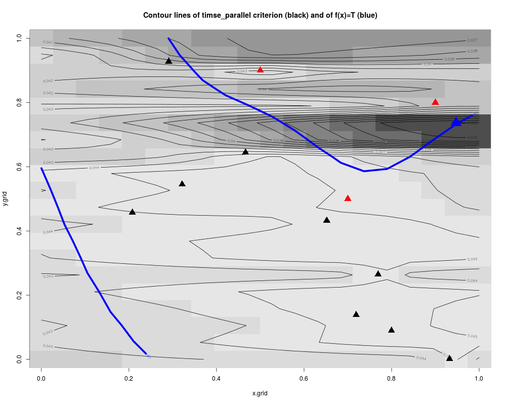
#plots: contour of the criterion, doe points and new point
image(x=x.grid,y=y.grid,z=z.grid,col=grey.colors(10))
contour(x=x.grid,y=y.grid,z=z.grid,15,add=TRUE)
points(design, col="black", pch=17, lwd=4,cex=2)
points(matrix(other.points,ncol=2,byrow=TRUE), col="red", pch=17, lwd=4,cex=2)

i.best <- which.min(timse_parallel.grid)
points(x[i.best,], col="blue", pch=17, lwd=4,cex=3)

#plots the real (unknown in practice) curve f(x)=T
testfun.grid <- apply(x,1,testfun)
z.grid.2 <- matrix(testfun.grid, n.grid, n.grid)
contour(x.grid,y.grid,z.grid.2,levels=T,col="blue",add=TRUE,lwd=5)
title("Contour lines of timse_parallel criterion (black) and of f(x)=T (blue)")

Results


R version 3.3.1 (2016-06-21) -- "Bug in Your Hair"
Copyright (C) 2016 The R Foundation for Statistical Computing
Platform: x86_64-pc-linux-gnu (64-bit)

R is free software and comes with ABSOLUTELY NO WARRANTY.
You are welcome to redistribute it under certain conditions.
Type 'license()' or 'licence()' for distribution details.

R is a collaborative project with many contributors.
Type 'contributors()' for more information and
'citation()' on how to cite R or R packages in publications.

Type 'demo()' for some demos, 'help()' for on-line help, or
'help.start()' for an HTML browser interface to help.
Type 'q()' to quit R.

> library(KrigInv)
Loading required package: DiceKriging
Loading required package: pbivnorm
Loading required package: rgenoud
##  rgenoud (Version 5.7-12.4, Build Date: 2015-07-19)
##  See http://sekhon.berkeley.edu/rgenoud for additional documentation.
##  Please cite software as:
##   Walter Mebane, Jr. and Jasjeet S. Sekhon. 2011.
##   ``Genetic Optimization Using Derivatives: The rgenoud package for R.''
##   Journal of Statistical Software, 42(11): 1-26. 
##

Loading required package: randtoolbox
Loading required package: rngWELL
This is randtoolbox. For overview, type 'help("randtoolbox")'.
> png(filename="/home/ddbj/snapshot/RGM3/R_CC/result/KrigInv/timse_optim_parallel2.Rd_%03d_medium.png", width=480, height=480)
> ### Name: timse_optim_parallel2
> ### Title: Parallel timse criterion
> ### Aliases: timse_optim_parallel2
> 
> ### ** Examples
> 
> #timse_optim_parallel2
> 
> set.seed(8)
> N <- 9 #number of observations
> T <- 80 #threshold
> testfun <- branin
> 
> #a 9 points initial design
> design <- data.frame( matrix(runif(2*N),ncol=2) )
> response <- testfun(design)
> 
> #km object with matern3_2 covariance
> #params estimated by ML from the observations
> model <- km(formula=~., design = design, 
+ 	response = response,covtype="matern3_2")

optimisation start
------------------
* estimation method   : MLE 
* optimisation method : BFGS 
* analytical gradient : used
* trend model : ~X1 + X2
* covariance model : 
  - type :  matern3_2 
  - nugget : NO
  - parameters lower bounds :  1e-10 1e-10 
  - parameters upper bounds :  1.448893 1.853021 
  - best initial criterion value(s) :  -25.38168 

N = 2, M = 5 machine precision = 2.22045e-16
At X0, 0 variables are exactly at the bounds
At iterate     0  f=       25.382  |proj g|=      0.19431
At iterate     1  f =       25.027  |proj g|=       0.13259
At iterate     2  f =       25.014  |proj g|=        1.6725
At iterate     3  f =       25.002  |proj g|=       0.15969
At iterate     4  f =       25.001  |proj g|=       0.17792
At iterate     5  f =       24.999  |proj g|=       0.31318
At iterate     6  f =       24.998  |proj g|=       0.14968
At iterate     7  f =       24.998  |proj g|=       0.03446
At iterate     8  f =       24.998  |proj g|=       0.03458
At iterate     9  f =       24.998  |proj g|=     0.0084816
At iterate    10  f =       24.998  |proj g|=      0.038393
At iterate    11  f =       24.997  |proj g|=        1.3196
At iterate    12  f =       24.997  |proj g|=        1.3327
At iterate    13  f =       24.994  |proj g|=        1.8077
At iterate    14  f =       24.991  |proj g|=        1.8106
At iterate    15  f =       24.975  |proj g|=        1.8136
At iterate    16  f =       24.937  |proj g|=        1.8202
At iterate    17  f =       24.816  |proj g|=        1.8136
At iterate    18  f =       24.652  |proj g|=       0.81261
At iterate    19  f =       24.652  |proj g|=       0.25743
At iterate    20  f =       24.651  |proj g|=     0.0033442
At iterate    21  f =       24.651  |proj g|=    1.4045e-05

iterations 21
function evaluations 30
segments explored during Cauchy searches 22
BFGS updates skipped 0
active bounds at final generalized Cauchy point 1
norm of the final projected gradient 1.40447e-05
final function value 24.6515

F = 24.6515
final  value 24.651471 
converged
> 
> ###we need to compute some additional arguments:
> #integration points, and current kriging means and variances at these points
> integcontrol <- list(n.points=1000,distrib="timse",init.distrib="MC")
> obj <- integration_design(integcontrol=integcontrol,lower=c(0,0),upper=c(1,1),
+ model=model,T=T)
> 
> integration.points <- obj$integration.points
> integration.weights <- obj$integration.weights
> pred <- predict_nobias_km(object=model,newdata=integration.points,
+ type="UK",se.compute=TRUE)
> intpoints.oldmean <- pred$mean ; intpoints.oldsd<-pred$sd
> 
> #another precomputation
> precalc.data <- precomputeUpdateData(model,integration.points)
> 
> #we also need to compute weights. Otherwise the (more simple) 
> #imse criterion will be evaluated
> weight <- 1/sqrt(2*pi*intpoints.oldsd^2) * 
+ exp(-0.5*((intpoints.oldmean-T)/sqrt(intpoints.oldsd^2))^2)
> weight[is.nan(weight)] <- 0
> 
> batchsize <- 4
> other.points <- c(0.7,0.5,0.5,0.9,0.9,0.8)
> x <- c(0.1,0.2)
> #one evaluation of the timse_optim_parallel criterion2
> #we calculate the expectation of the future "timse" uncertainty 
> #when 1+3 points are added to the doe
> #the 1+3 points are (0.1,0.2) and (0.7,0.5), (0.5,0.9), (0.9,0.8)
> timse_optim_parallel2(x=x,other.points,integration.points=integration.points,
+           integration.weights=integration.weights,
+           intpoints.oldmean=intpoints.oldmean,intpoints.oldsd=intpoints.oldsd,
+           precalc.data=precalc.data,T=T,model=model,weight=weight,
+           batchsize=batchsize,current.timse=Inf)
[1] 0.04396366
> 
> n.grid <- 20 #you can run it with 100
> x.grid <- y.grid <- seq(0,1,length=n.grid)
> x <- expand.grid(x.grid, y.grid)
> timse_parallel.grid <- apply(X=x,FUN=timse_optim_parallel2,MARGIN=1,other.points,
+           integration.points=integration.points,
+           integration.weights=integration.weights,
+           intpoints.oldmean=intpoints.oldmean,intpoints.oldsd=intpoints.oldsd,
+           precalc.data=precalc.data,T=T,model=model,weight=weight,
+           batchsize=batchsize,current.timse=Inf)
> z.grid <- matrix(timse_parallel.grid, n.grid, n.grid)
> 
> #plots: contour of the criterion, doe points and new point
> image(x=x.grid,y=y.grid,z=z.grid,col=grey.colors(10))
> contour(x=x.grid,y=y.grid,z=z.grid,15,add=TRUE)
> points(design, col="black", pch=17, lwd=4,cex=2)
> points(matrix(other.points,ncol=2,byrow=TRUE), col="red", pch=17, lwd=4,cex=2)
> 
> i.best <- which.min(timse_parallel.grid)
> points(x[i.best,], col="blue", pch=17, lwd=4,cex=3)
> 
> #plots the real (unknown in practice) curve f(x)=T
> testfun.grid <- apply(x,1,testfun)
> z.grid.2 <- matrix(testfun.grid, n.grid, n.grid)
> contour(x.grid,y.grid,z.grid.2,levels=T,col="blue",add=TRUE,lwd=5)
> title("Contour lines of timse_parallel criterion (black) and of f(x)=T (blue)")
> 
> 
> 
> 
> 
> dev.off()
null device 
          1 
>